


Tutorial
Contents
Introduction
Biotite is a Python package for computational biologists. It aims to provide a broad set of tools for working with different kinds of biological data, from sequences to structures. On the one hand side, working with Biotite should be computationally efficient, with the help of the powerful packages NumPy and Cython. On the other hand it aims for simple usability and extensibility, so that beginners are not overwhelmed and advanced users can easily build upon the existing system to implement their own algorithms.
Biotite provides 4 subpackages:
The biotite.sequence subpackage contains functionality for
working with sequence information of any kind.
The package contains by default sequence types for nucleotides and
proteins, but the alphabet-based implementation allows simple
integration of own sequence types, even if they do not rely on letters.
Beside the standard I/O operations, the package includes general purpose
functions for sequence manipulations and alignments.
The biotite.structure subpackage enables handling of 3D
structures of biomolecules.
Simplified, a structure is represented by a list of atoms and their
properties,
based on NumPy arrays.
The subpackage includes read/write functionality for different formats,
structure filters, coordinate transformations, angle and bond
measurements, structure
superimposition and some more advanced analysis capabilities.
The biotite.database subpackage is all about downloading data
from biological databases, including the probably most important ones:
the RCSB PDB and the NCBI Entrez database.
The biotite.application subpackage provides interfaces for
external software.
The interfaces range from locally installed software (e.g. MSA software)
to web applications (e.g. BLAST).
The speciality is that the interfaces are seamless:
You do not have to write input files and read output files, you only
have to input Python objects and you get Python objects.
It is basically very similar to using normal functions.
In the following sections you will get an overview over the mentioned subpackages, so go and grab some tea and cookies und let us begin.
Preliminary note
The files used in this tutorial will be stored in a temporary directory. So make sure to put the files, you want keep, somewhere else.
Data to work with - The Database subpackage
Biological databases are the backbone of computational biology.
The biotite.database subpackage provides interfaces for popular
online databases like the RCSB PDB or the NCBI Entrez database.
Fetching structure files from the RCSB PDB
Downloading structure files from the RCSB PDB is quite easy:
Simply specify the PDB ID, the file format and the target directory
for the fetch() function and you are done.
The function returns the path to the downloaded file, so you
can simply load the file via the other Biotite subpackages
(more on this later).
We will download on a protein structure of the miniprotein TC5b
(PDB: 1L2Y) into a temporary directory.
from tempfile import gettempdir
import biotite.database.rcsb as rcsb

file_path = rcsb.fetch("1l2y", "pdb", gettempdir())
print(file_path)
/tmp/1l2y.pdb
In case you want to download multiple files, you are able to specify a list of PDB IDs, which in return gives you a list of file paths.
# Download files in the more modern mmCIF format
file_paths = rcsb.fetch(["1l2y", "1aki"], "cif", gettempdir())
print([file_path for file_path in file_paths])
['/tmp/1l2y.cif', '/tmp/1aki.cif']
By default fetch() checks whether the file to be fetched
already exists in the directory and downloads it, if it does not
exist yet.
If you want to download files irrespectively, set overwrite to
true.
# Download file in the fast and small BinaryCIF format
file_path = rcsb.fetch("1l2y", "bcif", gettempdir(), overwrite=True)
If you omit the file path or set it to None, the downloaded data
will be returned directly as a file-like object, without creating a
file on your disk at all.
file = rcsb.fetch("1l2y", "pdb")
lines = file.readlines()
print("\n".join(lines[:10] + ["..."]))
HEADER    DE NOVO PROTEIN                         25-FEB-02   1L2Y

TITLE     NMR STRUCTURE OF TRP-CAGE MINIPROTEIN CONSTRUCT TC5B

COMPND    MOL_ID: 1;

COMPND   2 MOLECULE: TC5B;

COMPND   3 CHAIN: A;

COMPND   4 ENGINEERED: YES

SOURCE    MOL_ID: 1;

SOURCE   2 SYNTHETIC: YES;

SOURCE   3 OTHER_DETAILS: THE PROTEIN WAS SYNTHESIZED USING STANDARD FMOC

SOURCE   4 SOLID-PHASE SYNTHESIS METHODS ON AN APPLIED BIOSYSTEMS 433A PEPTIDE

...
In many cases you are not interested in a specific structure, but you
want a set of structures that fits your desired criteria.
For this purpose the RCSB search API can be used.
At first you have to create Query object for the property you
want to filter.
The search() method takes the Query and returns a
list of PDB IDs, which itself can be used as input for
fetch().
Likewise, count() is used to count the number of matching
PDB IDs.
query = rcsb.BasicQuery("HCN1")
pdb_ids = rcsb.search(query)
print(pdb_ids)
print(rcsb.count(query))
files = rcsb.fetch(pdb_ids, "cif", gettempdir())
['2XPI', '5U6O', '5U6P', '6UQF', '6UQG', '3U0Z']
6
This was a simple search for the occurrence of the search term in any
field.
You can also search for a value in a specific field with a
FieldQuery.
A complete list of the available fields and its supported operators
is documented
on this page
and on that page <https://search.rcsb.org/chemical-search-attributes.html>.
# Query for 'lacA' gene
query1 = rcsb.FieldQuery(
    "rcsb_entity_source_organism.rcsb_gene_name.value",
    exact_match="lacA"
)
# Query for resolution below 1.5 Å
query2 = rcsb.FieldQuery("reflns.d_resolution_high", less=1.5)
The search API allows even more complex queries, e.g. for sequence
or structure similarity. Have a look at the API reference of
biotite.database.rcsb.
Multiple Query objects can be combined using the | (or)
or & (and) operator for a more fine-grained selection.
A FieldQuery is negated with ~.
composite_query = query1 & ~query2
print(rcsb.search(composite_query))
['1KQA', '1KRR', '1KRU', '1KRV', '3U7V', '4DUW', '4IUG', '4LFK', '4LFL', '4LFM', '4LFN', '5IFP', '5IFT', '5IHR', '5JUV', '5MGC', '5MGD']
Often the structures behind the obtained PDB IDs have degree of
redundancy.
For example they may represent the same protein sequences or result
from the same set of experiments.
You may use Grouping of structures to group redundant
entries or even return only single representatives of each group.
query = rcsb.BasicQuery("Transketolase")
# Group PDB IDs from the same collection
print(rcsb.search(
    query, group_by=rcsb.DepositGrouping(), return_groups=True
))
# Get only a single representative of each group
print(rcsb.search(
    query, group_by=rcsb.DepositGrouping(), return_groups=False
))
{'G_1002178': ['5RW0', '5RVZ', '5RVY', '5RVX', '5RVW'], 'G_1002179': ['5RW1']}
['5RW0', '5RW1']
Note that grouping may omit PDB IDs in search results, if such PDB IDs cannot be grouped. In the example shown above, not all structures For example in the case shown above only a few PDB entries were uploaded as collection and hence are part of the search results.
Fetching files from the NCBI Entrez database
Another important source of biological information is the
NCBI Entrez database, which is commonly known as the NCBI.
It provides a myriad of information, ranging from sequences and
sequence features to scientific articles.
Fetching files from NCBI Entrez works analogous to the RCSB interface.
This time we have to provide the UIDs (Accession or GI) instead of
PDB IDs to the fetch() function.
Furthermore, we need to specifiy the database to retrieve the data
from and the retrieval type.
from tempfile import gettempdir, NamedTemporaryFile
import biotite.database.entrez as entrez

# Fetch a single UID ...
file_path = entrez.fetch(
    "NC_001416", gettempdir(), suffix="fa",
    db_name="nuccore", ret_type="fasta"
)
print(file_path)
# ... or multiple UIDs
file_paths = entrez.fetch(
    ["1L2Y_A","1AKI_A"], gettempdir(), suffix="fa",
    db_name="protein", ret_type="fasta"
)
print([file_path for file_path in file_paths])
/tmp/NC_001416.fa
['/tmp/1L2Y_A.fa', '/tmp/1AKI_A.fa']
A list of valid database, retrieval type and mode combinations can
be found
here.
Furthermore, get_database_name() can be helpful to get the
required database name by the more commonly known names.
print(entrez.get_database_name("Nucleotide"))
nuccore
The Entrez database allows for packing data for multiple UIDs into a
single file. This is achieved with the fetch_single_file()
function.
temp_file = NamedTemporaryFile(suffix=".fasta", delete=False)
file_path = entrez.fetch_single_file(
    ["1L2Y_A","1AKI_A"], temp_file.name, db_name="protein", ret_type="fasta"
)
print(file_path)
temp_file.close()
/tmp/tmp_lfoni2m.fasta
Similar to the RCSB PDB, you can also search every field of the NCBI Entrez database.
# Search in all fields
print(entrez.SimpleQuery("BL21 genome"))
# Search in the 'Organism' field
print(entrez.SimpleQuery("Escherichia coli", field="Organism"))
"BL21 genome"
"Escherichia coli"[Organism]
You can also combine multiple Query objects in any way you
like using the binary operators |, & and ^,
that represent OR, AND and NOT linkage, respectively.
composite_query = (
    entrez.SimpleQuery("50:100", field="Sequence Length") &
    (
        entrez.SimpleQuery("Escherichia coli", field="Organism") |
        entrez.SimpleQuery("Bacillus subtilis", field="Organism")
    )
)
print(composite_query)
(50:100[Sequence Length]) AND (("Escherichia coli"[Organism]) OR ("Bacillus subtilis"[Organism]))
Finally, the query is given to the search() function to obtain
the GIs, that can be used as input for fetch().
# Return a maximum number of 10 entries
gis = entrez.search(composite_query, "protein", number=10)
print(gis)
['2675477030', '2575482826', '2415618585', '2195794467', '2106033976', '1863112657', '1214787950', '1074718823', '1074718766', '921981618']
From A to T - The Sequence subpackage
biotite.sequence is a Biotite subpackage concerning maybe the
most popular type of data in bioinformatics: sequences.
The instantiation can be quite simple as
import biotite.sequence as seq
from biotite.sequence.align.matrix import SubstitutionMatrix

dna = seq.NucleotideSequence("AACTGCTA")
print(dna)
AACTGCTA
This example shows NucleotideSequence which is a subclass of
the abstract base class Sequence.
A NucleotideSequence accepts an iterable object of strings,
where each string can be 'A', 'C', 'G' or 'T'.
Each of these letters is called a symbol.
In general the sequence implementation in Biotite allows for
sequences of anything.
This means any immutable and hashable Python object can be used as
a symbol in a sequence, as long as the object is part of the
Alphabet of the particular Sequence.
An Alphabet object simply represents a list of objects that
are allowed to occur in a Sequence.
The following figure shows how the symbols are stored in a
Sequence object.

When setting the Sequence object with a sequence of symbols,
the Alphabet of the Sequence encodes each symbol in
the input sequence into a so called symbol code.
The encoding process is quite simple:
A symbol s is at index i in the list of allowed symbols in the
alphabet, so the symbol code for s is i.
If s is not in the alphabet, an AlphabetError is raised.
The array of symbol codes, that arises from encoding the input
sequence, is called sequence code.
This sequence code is now stored in an internal integer
ndarray in the Sequence object.
The sequence code is now accessed via the code attribute,
the corresponding symbols via the symbols attribute.
This approach has multiple advantages:
Ability to create sequences of anything
Sequence utility functions (searches, alignments,…) usually do not care about the specific sequence type, since they work with the internal sequence code
Integer type for sequence code is only as large as the alphabet requests
Sequence codes can be directly used as substitution matrix indices in alignments
Effectively, this means a potential Sequence subclass could
look like following:
class NonsenseSequence(seq.Sequence):

    alphabet = seq.Alphabet([42, "foo", b"bar"])

    def get_alphabet(self):
        return NonsenseSequence.alphabet

sequence = NonsenseSequence(["foo", b"bar", 42, "foo", "foo", 42])
print("Alphabet:", sequence.alphabet)
print("Symbols:", sequence.symbols)
print("Code:", sequence.code)
Alphabet: [42, 'foo', b'bar']
Symbols: ['foo', b'bar', 42, 'foo', 'foo', 42]
Code: [1 2 0 1 1 0]
From DNA to Protein
Biotite offers two prominent Sequence sublasses:
The NucleotideSequence represents DNA.
It may use two different alphabets - an unambiguous alphabet
containing the letters 'A', 'C', 'G' and 'T' and an
ambiguous alphabet containing additionally the standard letters for
ambiguous nucleic bases.
A NucleotideSequence determines automatically which alphabet
is required, unless an alphabet is specified. If you want to work with
RNA sequences you can use this class, too, you just need to replace
the 'U' with 'T'.
import biotite.sequence as seq

# Create a nucleotide sequence using a string
# The constructor can take any iterable object (e.g. a list of symbols)
seq1 = seq.NucleotideSequence("ACCGTATCAAG")
print(seq1.get_alphabet())
# Constructing a sequence with ambiguous nucleic bases
seq2 = seq.NucleotideSequence("TANNCGNGG")
print(seq2.get_alphabet())
['A', 'C', 'G', 'T']
['A', 'C', 'G', 'T', 'R', 'Y', 'W', 'S', 'M', 'K', 'H', 'B', 'V', 'D', 'N']
The reverse complement of a DNA sequence is created by chaining the
Sequence.reverse() and the
NucleotideSequence.complement() method.
# Lower case characters are automatically capitalized
seq1 = seq.NucleotideSequence("tacagtt")
print("Original:", seq1)
seq2 = seq1.reverse().complement()
print("Reverse complement:", seq2)
Original: TACAGTT
Reverse complement: AACTGTA
The other Sequence type is ProteinSequence.
It supports the letters for the 20 standard amino acids plus some
letters for ambiguous amino acids and a letter for a stop signal.
Furthermore, this class provides some utilities like
3-letter to 1-letter translation (and vice versa).
prot_seq = seq.ProteinSequence("BIQTITE")
print("-".join([seq.ProteinSequence.convert_letter_1to3(symbol)
                for symbol in prot_seq]))
ASX-ILE-GLN-THR-ILE-THR-GLU
A NucleotideSequence can be translated into a
ProteinSequence via the
NucleotideSequence.translate() method.
By default, the method searches for open reading frames (ORFs) in the
3 frames of the sequence.
A 6-frame ORF search requires an
additional call of NucleotideSequence.translate() with the
reverse complement of the sequence.
If you want to conduct a complete 1-frame translation of the sequence,
irrespective of any start and stop codons, set the parameter
complete to true.
dna = seq.NucleotideSequence("CATATGATGTATGCAATAGGGTGAATG")
proteins, pos = dna.translate()
for i in range(len(proteins)):
    print(
        f"Protein sequence {str(proteins[i])} "
        f"from base {pos[i][0]+1} to base {pos[i][1]}"
    )
protein = dna.translate(complete=True)
print("Complete translation:", str(protein))
Protein sequence MMYAIG* from base 4 to base 24
Protein sequence MYAIG* from base 7 to base 24
Protein sequence MQ* from base 11 to base 19
Protein sequence M from base 25 to base 27
Complete translation: HMMYAIG*M
The upper example uses the default CodonTable instance.
This can be changed with the codon_table parameter.
A CodonTable maps codons to amino acids and defines start
codons (both in symbol and code form).
A CodonTable is mainly used in the
NucleotideSequence.translate() method,
but can also be used to find the corresponding amino acid for a codon
and vice versa.
table = seq.CodonTable.default_table()
# Find the amino acid encoded by a given codon
print(table["TAC"])
# Find the codons encoding a given amino acid
print(table["Y"])
# Works also for codes instead of symbols
print(table[(1,2,3)])
print(table[14])
Y
('TAC', 'TAT')
14
((0, 2, 0), (0, 2, 2), (1, 2, 0), (1, 2, 1), (1, 2, 2), (1, 2, 3))
The default CodonTable is equal to the NCBI “Standard” table,
with the small difference that only 'ATG' qualifies as start
codon.
You can also use any other official NCBI table via
CodonTable.load().
# Use the official NCBI table name
table = seq.CodonTable.load("Yeast Mitochondrial")
print("Yeast Mitochondrial:")
print(table)
print()
# Use the official NCBI table ID
table = seq.CodonTable.load(11)
print("Bacterial:")
print(table)
Yeast Mitochondrial:
AAA K      AAC N      AAG K      AAT N
ACA T      ACC T      ACG T      ACT T
AGA R      AGC S      AGG R      AGT S
ATA M i    ATC I      ATG M i    ATT I

CAA Q      CAC H      CAG Q      CAT H
CCA P      CCC P      CCG P      CCT P
CGA R      CGC R      CGG R      CGT R
CTA T      CTC T      CTG T      CTT T

GAA E      GAC D      GAG E      GAT D
GCA A      GCC A      GCG A      GCT A
GGA G      GGC G      GGG G      GGT G
GTA V      GTC V      GTG V      GTT V

TAA *      TAC Y      TAG *      TAT Y
TCA S      TCC S      TCG S      TCT S
TGA W      TGC C      TGG W      TGT C
TTA L      TTC F      TTG L      TTT F

Bacterial:
AAA K      AAC N      AAG K      AAT N
ACA T      ACC T      ACG T      ACT T
AGA R      AGC S      AGG R      AGT S
ATA I i    ATC I i    ATG M i    ATT I

CAA Q      CAC H      CAG Q      CAT H
CCA P      CCC P      CCG P      CCT P
CGA R      CGC R      CGG R      CGT R
CTA L      CTC L      CTG L i    CTT L

GAA E      GAC D      GAG E      GAT D
GCA A      GCC A      GCG A      GCT A
GGA G      GGC G      GGG G      GGT G
GTA V      GTC V      GTG V i    GTT V

TAA *      TAC Y      TAG *      TAT Y
TCA S      TCC S      TCG S      TCT S
TGA *      TGC C      TGG W      TGT C
TTA L      TTC F      TTG L i    TTT F
Feel free to define your own custom codon table via the
CodonTable constructor.
Loading sequences from file
Biotite enables the user to load and save sequences from/to the
popular FASTA format via the FastaFile class.
A FASTA file may contain multiple sequences.
Each sequence entry starts with a line with a leading '>' and a
trailing header name.
The corresponding sequence is specified in the following lines until
the next header or end of file.
Since every sequence has its obligatory header, a FASTA file is
predestinated to be implemented as some kind of dictionary.
This is exactly what has been done in Biotite:
The header strings (without the '>') are used as keys to access
the respective sequence strings.
Actually you can cast the FastaFile object into a
dict.
Let’s demonstrate this on the genome of the lambda phage
(Accession: NC_001416).
After downloading the FASTA file from the NCBI Entrez database,
we can load its contents in the following way:
from tempfile import gettempdir, NamedTemporaryFile
import biotite.sequence as seq
import biotite.sequence.io.fasta as fasta
import biotite.database.entrez as entrez

file_path = entrez.fetch(
    "NC_001416", gettempdir(), suffix="fa",
    db_name="nuccore", ret_type="fasta"
)
fasta_file = fasta.FastaFile.read(file_path)
for header, string in fasta_file.items():
    print("Header:", header)
    print(len(string))
    print("Sequence:", string[:50], "...")
    print("Sequence length:", len(string))
Header: NC_001416.1 Enterobacteria phage lambda, complete genome
48502
Sequence: GGGCGGCGACCTCGCGGGTTTTCGCTATTTATGAAAATTTTCCGGTTTAA ...
Sequence length: 48502
Since there is only a single sequence in the file, the loop is run
only one time.
As the sequence string is very long, only the first 50 bp are printed.
Now this string could be used as input parameter for creation of a
NucleotideSequence.
But we want to spare ourselves some unnecessary work, there is already
a convenience function for that:
dna_seq = fasta.get_sequence(fasta_file)
print(type(dna_seq).__name__)
print(dna_seq[:50])
NucleotideSequence
GGGCGGCGACCTCGCGGGTTTTCGCTATTTATGAAAATTTTCCGGTTTAA
In this form get_sequence() returns the first sequence in the
file, which is also the only sequence in most cases.
If you want the sequence corresponding to a specific header, you have
to specifiy the header parameter.
The function even automatically recognizes, if the file contains a
DNA or protein sequence and returns a NucleotideSequence or
ProteinSequence, instance respectively.
Actually, it just tries to create a NucleotideSequence,
and if this fails, a ProteinSequence is created instead.
Sequences can be written into FASTA files in a similar way: either via
dictionary-like access or using the set_sequence()
convenience function.
# Create new empty FASTA file
fasta_file = fasta.FastaFile()
# PROTIP: Let your cat walk over the keyboard
dna_seq1 = seq.NucleotideSequence("ATCGGATCTATCGATGCTAGCTACAGCTAT")
dna_seq2 = seq.NucleotideSequence("ACGATCTACTAGCTGATGTCGTGCATGTACG")
# Append entries to file...
# ... via set_sequence()
fasta.set_sequence(fasta_file, dna_seq1, header="gibberish")
# .. or dictionary style
fasta_file["more gibberish"] = str(dna_seq2)
print(fasta_file)
temp_file = NamedTemporaryFile(suffix=".fasta", delete=False)
fasta_file.write(temp_file.name)
temp_file.close()
>gibberish
ATCGGATCTATCGATGCTAGCTACAGCTAT
>more gibberish
ACGATCTACTAGCTGATGTCGTGCATGTACG
As you see, our file contains our new 'gibberish' and
'more gibberish' sequences now.
In a similar manner sequences and sequence quality scores can be read
from FASTQ files. For further reference, have a look at the
biotite.sequence.io.fastq subpackage.
Alternatively, a sequence can also be loaded from GenBank or GenPept
files, using the GenBankFile class (more on this later).
Sequence search
A sequence can be searched for the position of a subsequence or a specific symbol:
import biotite.sequence as seq

main_seq = seq.NucleotideSequence("ACCGTATCAAGTATTG")
sub_seq = seq.NucleotideSequence("TAT")
print("Occurences of 'TAT':", seq.find_subsequence(main_seq, sub_seq))
print("Occurences of 'C':", seq.find_symbol(main_seq, "C"))
Occurences of 'TAT': [ 4 11]
Occurences of 'C': [1 2 7]
Sequence alignments
Pairwise alignments
When comparing two (or more) sequences, usually an alignment needs to be performed. Two kinds of algorithms need to be distinguished here: Heuristic algorithms do not guarantee to yield the optimal alignment, but instead they are very fast. On the other hand, there are algorithms that calculate the optimal (maximum similarity score) alignment, but are quite slow.
The biotite.sequence.align package provides the function
align_optimal(), which fits into the latter category.
It either performs an optimal global alignment, using the
Needleman-Wunsch algorithm, or an optimal local
alignment, using the Smith-Waterman algorithm.
By default it uses a linear gap penalty, but an affine gap penalty
can be used, too.
Most functions in biotite.sequence.align can align any two
Sequence objects with each other.
In fact the Sequence objects can be instances from different
Sequence subclasses and therefore may have different
alphabets.
The only condition that must be satisfied, is that the
SubstitutionMatrix alphabets match the alphabets of the
sequences to be aligned.
But wait, what’s a SubstitutionMatrix?
This class maps a combination of two symbols, one from the first
sequence the other one from the second sequence, to a similarity
score.
A SubstitutionMatrix object contains two alphabets with
length n or m, respectively, and an (n,m)-shaped
ndarray storing the similarity scores.
You can choose one of many predefined matrices from an internal
database or you can create a custom matrix on your own.
So much for theory.
Let’s start by showing different ways to construct a
SubstitutionMatrix, in our case for protein sequence
alignments:
import biotite.sequence as seq
import biotite.sequence.align as align
import numpy as np

alph = seq.ProteinSequence.alphabet
# Load the standard protein substitution matrix, which is BLOSUM62
matrix = align.SubstitutionMatrix.std_protein_matrix()
print("\nBLOSUM62\n")
print(matrix)
# Load another matrix from internal database
matrix = align.SubstitutionMatrix(alph, alph, "BLOSUM50")
# Load a matrix dictionary representation,
# modify it, and create the SubstitutionMatrix
# (The dictionary could be alternatively loaded from a string containing
# the matrix in NCBI format)
matrix_dict = align.SubstitutionMatrix.dict_from_db("BLOSUM62")
matrix_dict[("P","Y")] = 100
matrix = align.SubstitutionMatrix(alph, alph, matrix_dict)
# And now create a matrix by directly provding the ndarray
# containing the similarity scores
# (identity matrix in our case)
scores = np.identity(len(alph), dtype=int)
matrix = align.SubstitutionMatrix(alph, alph, scores)
print("\n\nIdentity matrix\n")
print(matrix)
BLOSUM62

    A   C   D   E   F   G   H   I   K   L   M   N   P   Q   R   S   T   V   W   Y   B   Z   X   *
A   4   0  -2  -1  -2   0  -2  -1  -1  -1  -1  -2  -1  -1  -1   1   0   0  -3  -2  -2  -1   0  -4
C   0   9  -3  -4  -2  -3  -3  -1  -3  -1  -1  -3  -3  -3  -3  -1  -1  -1  -2  -2  -3  -3  -2  -4
D  -2  -3   6   2  -3  -1  -1  -3  -1  -4  -3   1  -1   0  -2   0  -1  -3  -4  -3   4   1  -1  -4
E  -1  -4   2   5  -3  -2   0  -3   1  -3  -2   0  -1   2   0   0  -1  -2  -3  -2   1   4  -1  -4
F  -2  -2  -3  -3   6  -3  -1   0  -3   0   0  -3  -4  -3  -3  -2  -2  -1   1   3  -3  -3  -1  -4
G   0  -3  -1  -2  -3   6  -2  -4  -2  -4  -3   0  -2  -2  -2   0  -2  -3  -2  -3  -1  -2  -1  -4
H  -2  -3  -1   0  -1  -2   8  -3  -1  -3  -2   1  -2   0   0  -1  -2  -3  -2   2   0   0  -1  -4
I  -1  -1  -3  -3   0  -4  -3   4  -3   2   1  -3  -3  -3  -3  -2  -1   3  -3  -1  -3  -3  -1  -4
K  -1  -3  -1   1  -3  -2  -1  -3   5  -2  -1   0  -1   1   2   0  -1  -2  -3  -2   0   1  -1  -4
L  -1  -1  -4  -3   0  -4  -3   2  -2   4   2  -3  -3  -2  -2  -2  -1   1  -2  -1  -4  -3  -1  -4
M  -1  -1  -3  -2   0  -3  -2   1  -1   2   5  -2  -2   0  -1  -1  -1   1  -1  -1  -3  -1  -1  -4
N  -2  -3   1   0  -3   0   1  -3   0  -3  -2   6  -2   0   0   1   0  -3  -4  -2   3   0  -1  -4
P  -1  -3  -1  -1  -4  -2  -2  -3  -1  -3  -2  -2   7  -1  -2  -1  -1  -2  -4  -3  -2  -1  -2  -4
Q  -1  -3   0   2  -3  -2   0  -3   1  -2   0   0  -1   5   1   0  -1  -2  -2  -1   0   3  -1  -4
R  -1  -3  -2   0  -3  -2   0  -3   2  -2  -1   0  -2   1   5  -1  -1  -3  -3  -2  -1   0  -1  -4
S   1  -1   0   0  -2   0  -1  -2   0  -2  -1   1  -1   0  -1   4   1  -2  -3  -2   0   0   0  -4
T   0  -1  -1  -1  -2  -2  -2  -1  -1  -1  -1   0  -1  -1  -1   1   5   0  -2  -2  -1  -1   0  -4
V   0  -1  -3  -2  -1  -3  -3   3  -2   1   1  -3  -2  -2  -3  -2   0   4  -3  -1  -3  -2  -1  -4
W  -3  -2  -4  -3   1  -2  -2  -3  -3  -2  -1  -4  -4  -2  -3  -3  -2  -3  11   2  -4  -3  -2  -4
Y  -2  -2  -3  -2   3  -3   2  -1  -2  -1  -1  -2  -3  -1  -2  -2  -2  -1   2   7  -3  -2  -1  -4
B  -2  -3   4   1  -3  -1   0  -3   0  -4  -3   3  -2   0  -1   0  -1  -3  -4  -3   4   1  -1  -4
Z  -1  -3   1   4  -3  -2   0  -3   1  -3  -1   0  -1   3   0   0  -1  -2  -3  -2   1   4  -1  -4
X   0  -2  -1  -1  -1  -1  -1  -1  -1  -1  -1  -1  -2  -1  -1   0   0  -1  -2  -1  -1  -1  -1  -4
*  -4  -4  -4  -4  -4  -4  -4  -4  -4  -4  -4  -4  -4  -4  -4  -4  -4  -4  -4  -4  -4  -4  -4   1


Identity matrix

    A   C   D   E   F   G   H   I   K   L   M   N   P   Q   R   S   T   V   W   Y   B   Z   X   *
A   1   0   0   0   0   0   0   0   0   0   0   0   0   0   0   0   0   0   0   0   0   0   0   0
C   0   1   0   0   0   0   0   0   0   0   0   0   0   0   0   0   0   0   0   0   0   0   0   0
D   0   0   1   0   0   0   0   0   0   0   0   0   0   0   0   0   0   0   0   0   0   0   0   0
E   0   0   0   1   0   0   0   0   0   0   0   0   0   0   0   0   0   0   0   0   0   0   0   0
F   0   0   0   0   1   0   0   0   0   0   0   0   0   0   0   0   0   0   0   0   0   0   0   0
G   0   0   0   0   0   1   0   0   0   0   0   0   0   0   0   0   0   0   0   0   0   0   0   0
H   0   0   0   0   0   0   1   0   0   0   0   0   0   0   0   0   0   0   0   0   0   0   0   0
I   0   0   0   0   0   0   0   1   0   0   0   0   0   0   0   0   0   0   0   0   0   0   0   0
K   0   0   0   0   0   0   0   0   1   0   0   0   0   0   0   0   0   0   0   0   0   0   0   0
L   0   0   0   0   0   0   0   0   0   1   0   0   0   0   0   0   0   0   0   0   0   0   0   0
M   0   0   0   0   0   0   0   0   0   0   1   0   0   0   0   0   0   0   0   0   0   0   0   0
N   0   0   0   0   0   0   0   0   0   0   0   1   0   0   0   0   0   0   0   0   0   0   0   0
P   0   0   0   0   0   0   0   0   0   0   0   0   1   0   0   0   0   0   0   0   0   0   0   0
Q   0   0   0   0   0   0   0   0   0   0   0   0   0   1   0   0   0   0   0   0   0   0   0   0
R   0   0   0   0   0   0   0   0   0   0   0   0   0   0   1   0   0   0   0   0   0   0   0   0
S   0   0   0   0   0   0   0   0   0   0   0   0   0   0   0   1   0   0   0   0   0   0   0   0
T   0   0   0   0   0   0   0   0   0   0   0   0   0   0   0   0   1   0   0   0   0   0   0   0
V   0   0   0   0   0   0   0   0   0   0   0   0   0   0   0   0   0   1   0   0   0   0   0   0
W   0   0   0   0   0   0   0   0   0   0   0   0   0   0   0   0   0   0   1   0   0   0   0   0
Y   0   0   0   0   0   0   0   0   0   0   0   0   0   0   0   0   0   0   0   1   0   0   0   0
B   0   0   0   0   0   0   0   0   0   0   0   0   0   0   0   0   0   0   0   0   1   0   0   0
Z   0   0   0   0   0   0   0   0   0   0   0   0   0   0   0   0   0   0   0   0   0   1   0   0
X   0   0   0   0   0   0   0   0   0   0   0   0   0   0   0   0   0   0   0   0   0   0   1   0
*   0   0   0   0   0   0   0   0   0   0   0   0   0   0   0   0   0   0   0   0   0   0   0   1
For our protein alignment we will use the standard BLOSUM62 matrix.
seq1 = seq.ProteinSequence("BIQTITE")
seq2 = seq.ProteinSequence("IQLITE")
matrix = align.SubstitutionMatrix.std_protein_matrix()
print("\nLocal alignment")
alignments = align.align_optimal(seq1, seq2, matrix, local=True)
for ali in alignments:
    print(ali)
print("Global alignment")
alignments = align.align_optimal(seq1, seq2, matrix, local=False)
for ali in alignments:
    print(ali)
Local alignment
IQTITE
IQLITE
Global alignment
BIQTITE
-IQLITE
The alignment functions return a list of Alignment objects.
This object saves the input sequences together with a so called trace
- the indices to symbols in these sequences that are aligned to each
other (-1 for a gap).
Additionally the alignment score is stored in this object.
Furthermore, this object can prettyprint the alignment into a human
readable form.
For publication purposes you can create an actual figure based on Matplotlib. You can either decide to color the symbols based on the symbol type or based on the similarity within the alignment columns. In this case we will go with the similarity visualization.
import matplotlib.pyplot as plt
import biotite.sequence.graphics as graphics

fig, ax = plt.subplots(figsize=(2.0, 0.8))
graphics.plot_alignment_similarity_based(
    ax, alignments[0], matrix=matrix, symbols_per_line=len(alignments[0])
)
fig.tight_layout()

If you are interested in more advanced visualization examples, have a look at the example gallery.
You can also do some simple analysis on these objects, like determining the sequence identity or calculating the score. For further custom analysis, it can be convenient to have directly the aligned symbols codes instead of the trace.
alignment = alignments[0]
print("Score: ", alignment.score)
print("Recalculated score:", align.score(alignment, matrix=matrix))
print("Sequence identity:", align.get_sequence_identity(alignment))
print("Symbols:")
print(align.get_symbols(alignment))
print("symbols codes:")
print(align.get_codes(alignment))
Score:  12
Recalculated score: 12
Sequence identity: 0.8333333333333334
Symbols:
[['B', 'I', 'Q', 'T', 'I', 'T', 'E'], [None, 'I', 'Q', 'L', 'I', 'T', 'E']]
symbols codes:
[[20  7 13 16  7 16  3]
 [-1  7 13  9  7 16  3]]
You might wonder, why you should recalculate the score, when the score
has already been directly calculated via align_optimal().
The answer is that you might load an alignment from a FASTA file
using get_alignment(), where the score is not provided.
Advanced sequence alignments
While the former alignment method returns the optimal alignment of two sequences, it is not recommended to use this method to align a short query sequence (e.g a gene) to an extremely long sequence (e.g. the human genome): The computation time and memory space requirements scale linearly with the length of both sequences, so even if your RAM does not overflow, you might need to wait a very long time for your alignment results.
But there is another method: You could look for local k-mer matches of the long (reference) sequence and the short (query) sequence and perform a sequence alignment restricted to the position of the match. Although this approach might not give the optimal result in some cases, it works well enough, so that popular programs like BLAST are based on it.
Biotite provides a modular system to build such an alignment search method yourself. At least four steps are necessary:
Creating an index table mapping k-mers to their position in the reference sequence
Find match positions between this k-mer index table and the k-mers of the query sequence
Perform gapped alignments restricted to the match positions
Evaluate the significance of the created alignments
In the following example the short query protein sequence BIQTITE
is aligned to a longer reference sequence containing the ‘homologous’
NIQBITE in its middle.
While both sequences are relatively short and they could be easily
aligned with the align_optimal() function, the following
general approach scales well for real world applications, where the
reference could be a large genome or where you have a database of
thousands of sequences.
query = seq.ProteinSequence("BIQTITE")
reference = seq.ProteinSequence(
    # This toy sequence is adapted from the first sentence of the
    # Wikipedia 'Niobite' article
    "CQLVMBITEALSQCALLEDNIQBITEANDCQLVMBATEISAMINERALGRQVPTHATISANQREQFNIQBIVM"
    #                   ^^^^^^^
    # Here is the 'homologous' mineral
)
1. Indexing the reference sequence
In the first step the k-mers of the reference sequence needs to be
indexed into a KmerTable.
The k-mers (also called words or k-tuples) of a sequence are all
overlapping subsequences with a given length k.
Indexing means creating a table that maps each k-mer to the position
where this k-mer appears in the sequence - similar to the index of a
book.
Here the first decision needs to be made:
Which k is desired?
A small k improves the sensitivity, a large k decreases the
computation time in the later steps.
In this case we choose 3-mers.
# Create a k-mer index table from the k-mers of the reference sequence
kmer_table = align.KmerTable.from_sequences(
    # Use 3-mers
    k=3,
    # Add only the reference sequence to the table
    sequences=[reference],
    # The purpose of the reference ID is to identify the sequence
    ref_ids=[0]
)
The purpose of the reference ID is to identify not only the position of a k-mer in a sequence, but also which sequence is involved, if you add multiple sequences to the table. In this case there is only a single sequence in the table, so the reference ID is arbitrary.
Let’s have a deeper look under the hood:
The KmerTable creates a KmerAlphabet that encodes a
k-mer symbol, i.e. a tuple of k symbols from the base alphabet,
into a k-mer code.
Importantly, this k-mer code can be uniquely decoded back into
a k-mer symbol.
# Access the internal *k-mer* alphabet.
kmer_alphabet = kmer_table.kmer_alphabet
print("Base alphabet:", kmer_alphabet.base_alphabet)
print("k:", kmer_alphabet.k)
print("k-mer code for 'BIQ':", kmer_alphabet.encode("BIQ"))
Base alphabet: ['A', 'C', 'D', 'E', 'F', 'G', 'H', 'I', 'K', 'L', 'M', 'N', 'P', 'Q', 'R', 'S', 'T', 'V', 'W', 'Y', 'B', 'Z', 'X', '*']
k: 3
k-mer code for 'BIQ': 11701
for code in range(5):
    print(kmer_alphabet.decode(code))
print("...")
['A' 'A' 'A']
['A' 'A' 'C']
['A' 'A' 'D']
['A' 'A' 'E']
['A' 'A' 'F']
...
Furthermore the KmerAlphabet can encode all overlapping
k-mers of a sequence.
kmer_codes = kmer_alphabet.create_kmers(seq.ProteinSequence("BIQTITE").code)
print("k-mer codes:", kmer_codes)
print("k-mers:")
for kmer in kmer_alphabet.decode_multiple(kmer_codes):
    print("".join(kmer))
k-mer codes: [11701  4360  7879  9400  4419]
k-mers:
BIQ
IQT
QTI
TIT
ITE
Now we get back to the KmerTable.
When the table is created, it uses KmerAlphabet.create_kmers()
to get all k-mers in the sequence and stores for each k-mer the
position(s) where the respective k-mer appears.
# Get all positions for the 'ITE' k-mer
for ref_id, position in kmer_table[kmer_alphabet.encode("ITE")]:
    print(position)
6
23
2. Matching the query sequence
In the second step we would like to find k-mer matches of our
reference KmerTable with the query sequence.
A match is a k-mer that appears in both, the table and the query
sequence.
The KmerTable.match() method iterates over all
overlapping k-mers in the query and checks whether the
KmerTable has at least one position for this k-mer.
If it does, it adds the position in the query and all corresponding
positions saved in the KmerTable to the matches.
matches = kmer_table.match(query)
# Filter out the reference ID, because we have only one sequence
# in the table anyway
matches = matches[:, [0,2]]
for query_pos, ref_pos in matches:
    print(f"Match at query position {query_pos}, reference position {ref_pos}")
    # Print the reference sequence at the match position including four
    # symbols before and after the matching k-mer
    print("...", reference[ref_pos - 4 : ref_pos + kmer_table.k + 4], "...")
    print()
Match at query position 4, reference position 6
... LVMBITEALSQ ...

Match at query position 4, reference position 23
... NIQBITEANDC ...
We see that the 'ITE' of 'BIQTITE' matches the 'ITE' of
'CQLVMBITE' and 'NIQBITE'.
3. Alignments at the match positions
Now that we have found the match positions, we can perform an
alignment restricted to each match position.
Currently Biotite offers three functions for this purpose:
align_local_ungapped(), align_local_gapped() and
align_banded().
align_local_ungapped() and align_local_gapped()
perform fast local alignments expanding from a given seed position,
which is typically set to a match position from the previous step.
The alignment stops, if the current similarity score drops a given
threshold below the maximum score already found, a technique that is
also called X-Drop.
While align_local_ungapped() is much faster than
align_local_gapped(), it does not insert gaps into the
alignment.
In contrast align_banded() performs a local or global
alignment, where the alignment space is restricted to a defined
diagonal band, allowing only a certain number of insertions/deletions
in each sequence.
The presented methods have in common, that they ideally only traverse
through a small fraction of the possible alignment space, allowing
them to run much faster than align_optimal().
However they might not find the optimal alignment, if such an
alignment would have an intermediate low scoring region or too many
gaps in either sequence, respectively.
In this tutorial we will focus on using align_banded() to
perform a global alignment of our two sequences.
align_banded() requires two diagonals that define the lower
and upper limit of the alignment band.
A diagonal is an integer defined as \(D = j - i\), where i and
j are sequence positions in the first and second sequence,
respectively.
This means that two symbols at position i and j can only be
aligned to each other, if \(D_L \leq j - i \leq D_U\).
In our case we center the diagonal band to the diagonal of the match and use a fixed band width \(W = D_U - D_L\).
BAND_WIDTH = 4

matrix = SubstitutionMatrix.std_protein_matrix()
alignments = []
for query_pos, ref_pos in matches:
    diagonal = ref_pos - query_pos
    alignment = align.align_banded(
        query, reference, matrix, gap_penalty=-5, max_number=1,
        # Center the band at the match diagonal and extend the band by
        # one half of the band width in each direction
        band=(diagonal - BAND_WIDTH//2, diagonal + BAND_WIDTH//2)
    )[0]
    alignments.append(alignment)

for alignment in alignments:
    print(alignment)
    print("\n")
BIQTITE
LVMBITE


BIQTITE
NIQBITE
4. Significance evaluation
We have obtained two alignments, but which one of them is the
‘correct’ one?
in this simple example we could simply select the one with the highest
similarity score, but this approach is not sound in general:
A reference sequence might contain multiple regions, that are
homologous to the query, or none at all.
A better approach is a statistical measure, like the
BLAST E-value.
It gives the number of alignments expected by chance with a score at
least as high as the score obtained from the alignment of interest.
Hence, a value close to zero means a very significant homology.
We can calculate the E-value using the EValueEstimator, that
needs to be initialized with the same scoring scheme used for our
alignments.
For the sake of simplicity we choose uniform background frequencies
for each symbol, but usually you would choose values that reflect
the amino acid/nucleotide composition in your sequence database.
estimator = align.EValueEstimator.from_samples(
    seq.ProteinSequence.alphabet, matrix, gap_penalty=-5,
    frequencies=np.ones(len(seq.ProteinSequence.alphabet)),
    # Trade accuracy for a lower runtime
    sample_length=200
)
Now we can calculate the E-value for the alignments. Since we have aligned the query only to the reference sequence shown above, we use its length to calculate the E-value. If you have an entire sequence database you align against, you would take the total sequence length of the database instead.
scores = [alignment.score for alignment in alignments]
evalues = 10 ** estimator.log_evalue(scores, len(query), len(reference))
for alignment, evalue in zip(alignments, evalues):
    print(f"E-value = {evalue:.2e}")
    print(alignment)
    print("\n")
E-value = 6.78e-01
BIQTITE
LVMBITE


E-value = 3.94e-02
BIQTITE
NIQBITE
Finally, we can see that the expected alignment of BIQTITE to
NIQBITE is more significant than the unspecific match.
The setup shown here is a very simple one compared to the methods popular software like BLAST use. Since the k-mer matching step is very fast and the gapped alignments take the largest part of the time, you usually want to have additional filters before you trigger a gapped alignment: Commonly a gapped alignment is only started at a match, if there is another match on the same diagonal in proximity and if a fast local ungapped alignment (seed extension) exceeds a defined threshold score. Furthermore, the parameter selection, e.g. the k-mer length, is key to a fast but also sensitive alignment procedure. However, you can find suitable parameters in literature or run benchmarks by yourself to find appropriate parameters for your application.
Multiple sequence alignments
If you want to perform a multiple sequence alignment (MSA), have a
look at the align_multiple() function:
seq1 = seq.ProteinSequence("BIQTITE")
seq2 = seq.ProteinSequence("TITANITE")
seq3 = seq.ProteinSequence("BISMITE")
seq4 = seq.ProteinSequence("IQLITE")
alignment, order, guide_tree, distance_matrix = align.align_multiple(
    [seq1, seq2, seq3, seq4],
    matrix=align.SubstitutionMatrix.std_protein_matrix(),
    gap_penalty=-5,
    terminal_penalty=False
)
print(alignment)
BIQT-ITE
TITANITE
BISM-ITE
-IQL-ITE
This function is only recommended for strongly related sequences or
exotic sequence types.
When high accuracy or computation time matters, other MSA programs
deliver better results.
External MSA software can accessed via the biotite.application
subpackage.
Sequence features
Sequence features describe functional parts of a sequence,
like coding regions or regulatory parts.
One popular source to obtain information about sequence features are
GenBank (for DNA and RNA) and GenPept (for peptides) files.
As example for sequence features we will work with the GenBank file
for the avidin gene (Accession: AJ311647),
that we can download from the NCBI Entrez database.
After downloading we can load the file using the GenBankFile
class from biotite.sequence.io.genbank.
Similar to the other file classes we have encountered, a
GenBankFile provides a low-level interface.
In contrast, the biotite.sequence.io.genbank module contains
high-level functions to directly obtain useful objects from a
GenBankFile object.
import biotite.sequence.io.genbank as gb

file_path = entrez.fetch(
    "AJ311647", gettempdir(), suffix="gb",
    db_name="nuccore", ret_type="gb"
)
file = gb.GenBankFile.read(file_path)
print("Accession:", gb.get_accession(file))
print("Definition:", gb.get_definition(file))
Accession: AJ311647
Definition: Gallus gallus AVD gene for avidin, exons 1-4.
Now that we have loaded the file, we want to have a look at the
sequence features.
Therefore, we grab the Annotation from the file.
An annotation is the collection of features corresponding to one
sequence (the sequence itself is not included, though).
This Annotation can be iterated in order to obtain single
Feature objects.
Each Feature contains 3 pieces of information: Its feature
key (e.g. regulatory or CDS), a dictionary of qualifiers and
one or multiple locations on the corresponding sequence.
A Location in turn, contains its starting and its ending
base/residue position, the strand it is on (only for DNA) and possible
location defects (defects will be discussed later).
In the next example we will print the keys of the features and their
locations:
annotation = gb.get_annotation(file)
for feature in annotation:
    # Convert the feature locations in better readable format
    locs = [str(loc) for loc in sorted(feature.locs, key=lambda l: l.first)]
    print(f"{feature.key:12}   {locs}")
intron         ['1020-1106 >']
exon           ['1107-1152 >']
regulatory     ['26-33 >']
mRNA           ['98-178 >', '263-473 >', '899-1019 >', '1107-1152 >']
source         ['1-1224 >']
exon           ['98-178 >']
regulatory     ['1215-1220 >']
exon           ['899-1019 >']
exon           ['263-473 >']
gene           ['98-1152 >']
intron         ['179-262 >']
CDS            ['98-178 >', '263-473 >', '899-1019 >', '1107-1152 >']
intron         ['474-898 >']
sig_peptide    ['98-169 >']
The '>' characters in the string representations of a location
indicate that the location is on the forward strand.
Most of the features have only one location, except the mRNA and
CDS feature, which have 4 locations joined.
When we look at the rest of the features, this makes sense: The gene
has 4 exons.
Therefore, the mRNA (and consequently the CDS) is composed of
these exons.
The two regulatory features are the TATA box and the
poly-A signal, as the feature qualifiers make clear:
for feature in annotation:
    if feature.key == "regulatory":
        print(feature.qual["regulatory_class"])
TATA_box
polyA_signal_sequence
Similarily to Alignment objects, we can visualize an
Annotation using the biotite.sequence.graphics subpackage, in
a so called feature map.
In order to avoid overlaping features, we draw only the CDS feature.
# Get the range of the entire annotation via the *source* feature
for feature in annotation:
    if feature.key == "source":
        # loc_range has exclusive stop
        loc = list(feature.locs)[0]
        loc_range = (loc.first, loc.last+1)
fig, ax = plt.subplots(figsize=(8.0, 1.0))
graphics.plot_feature_map(
    ax,
    seq.Annotation(
        [feature for feature in annotation if feature.key == "CDS"]
    ),
    multi_line=False,
    loc_range=loc_range,
    show_line_position=True
)
fig.tight_layout()

Annotation objects can be indexed with slices, that represent
the start and the exclusive stop base/residue of the annotation from
which the subannotation is created.
All features, that are not in this range, are not included in the
subannotation.
In order to demonstrate this indexing method, we create a
subannotation that includes only features in range of the gene itself
(without the regulatory stuff).
# At first we have the find the feature with the 'gene' key
for feature in annotation:
    if feature.key == "gene":
        gene_feature = feature
# Then we create a subannotation from the feature's location
# Since the stop value of the slice is still exclusive,
# the stop value is the position of the last base +1
loc = list(gene_feature.locs)[0]
sub_annot = annotation[loc.first : loc.last +1]
# Print the remaining features and their locations
for feature in sub_annot:
    locs = [str(loc) for loc in sorted(feature.locs, key=lambda l: l.first)]
    print(f"{feature.key:12}   {locs}")
intron         ['1020-1106 >']
source         ['98-1152 >']
exon           ['1107-1152 >']
mRNA           ['98-178 >', '263-473 >', '899-1019 >', '1107-1152 >']
exon           ['98-178 >']
exon           ['899-1019 >']
exon           ['263-473 >']
gene           ['98-1152 >']
intron         ['179-262 >']
CDS            ['98-178 >', '263-473 >', '899-1019 >', '1107-1152 >']
intron         ['474-898 >']
sig_peptide    ['98-169 >']
The regulatory sequences have disappeared in the subannotation.
Another interesting thing happened:
The location of the source` feature narrowed and
is in range of the slice now. This happened, because the feature was
truncated:
The bases that were not in range of the slice were removed.
Let’s have a closer look into location defects now:
A Location instance has a defect, when the feature itself is
not directly located in the range of the first to the last base,
for example when the exact postion is not known or, as in our case, a
part of the feature was truncated.
Let’s have a closer look at the location defects of our subannotation:
for feature in sub_annot:
    defects = [str(location.defect) for location
               in sorted(feature.locs, key=lambda l: l.first)]
    print(f"{feature.key:12}   {defects}")
intron         ['Defect.NONE']
source         ['Defect.MISS_RIGHT|MISS_LEFT']
exon           ['Defect.NONE']
mRNA           ['Defect.BEYOND_LEFT', 'Defect.NONE', 'Defect.NONE', 'Defect.BEYOND_RIGHT']
exon           ['Defect.NONE']
exon           ['Defect.NONE']
exon           ['Defect.NONE']
gene           ['Defect.BEYOND_RIGHT|BEYOND_LEFT']
intron         ['Defect.NONE']
CDS            ['Defect.NONE', 'Defect.NONE', 'Defect.NONE', 'Defect.NONE']
intron         ['Defect.NONE']
sig_peptide    ['Defect.NONE']
The class Location.Defect is a Flag.
This means that multiple defects can be combined to one value.
NONE means that the location has no defect, which is true for most
of the features.
The source feature has a defect - a combination of MISS_LEFT
and MISS_RIGHT. MISS_LEFT is applied, if a feature was
truncated before the first base, and MISS_RIGHT is applied, if
a feature was truncated after the last base.
Since source` was truncated from both sides, the combination is
applied.
gene has the defect values BEYOND_LEFT and BEYOND_RIGHT.
These defects already appear in the GenBank file, since
the gene is defined as the unit that is transcribed into one
(pre-)mRNA.
As the transcription starts somewhere before the start of the coding
region and the exact start location is not known, BEYOND_LEFT is
applied.
In an analogous way, the transcription does stop somewhere after the
coding region (at the terminator signal).
Hence, BEYOND_RIGHT is applied.
These two defects are also reflected in the mRNA feature.
Annotated sequences
Now, that you have understood what annotations are, we proceed to the
next topic: annotated sequences.
An AnnotatedSequence is like an annotation, but the sequence
is included this time.
Since our GenBank file contains the
sequence corresponding to the feature table, we can directly obtain the
AnnotatedSequence.
annot_seq = gb.get_annotated_sequence(file)
print("Same annotation as before?", (annotation == annot_seq.annotation))
print(annot_seq.sequence[:60], "...")
Same annotation as before? True
ACTGGGCAGAGTCAGTGCTGGAAGCAATMAAAAGGCGAGGGAGCAGGCAGGGGTGAGTCC ...
When indexing an AnnotatedSequence with a slice,
the index is applied to the Annotation and the
Sequence.
While the Annotation handles the index as shown before,
the Sequence is indexed based on the sequence start
value (usually 1).
print("Sequence start before indexing:", annot_seq.sequence_start)
for feature in annot_seq.annotation:
    if feature.key == "regulatory" \
        and feature.qual["regulatory_class"] == "polyA_signal_sequence":
            polya_feature = feature
loc = list(polya_feature.locs)[0]
# Get annotated sequence containing only the poly-A signal region
poly_a = annot_seq[loc.first : loc.last +1]
print("Sequence start after indexing:", poly_a.sequence_start)
print(poly_a.sequence)
Sequence start before indexing: 1
Sequence start after indexing: 1215
AATAAA
Here we get the poly-A signal Sequence 'AATAAA'.
As you might have noticed, the sequence start has shifted to the start
of the slice index (the first base of the regulatory feature).
Warning
Since AnnotatedSequence objects use base position
indices and Sequence objects use array position indices,
you will get different results for annot_seq[n:m].sequence and
annot_seq.sequence[n:m].
There is also a convenient way to obtain the sequence corresponding to
a feature, even if the feature contains multiple locations or a
location is on the reverse strand:
Simply use a Feature object (in this case the CDS feature)
as index.
for feature in annot_seq.annotation:
    if feature.key == "CDS":
        cds_feature = feature
cds_seq = annot_seq[cds_feature]
print(cds_seq[:60], "...")
ATGGTGCACGCAACCTCCCCGCTGCTGCTGCTGCTGCTGCTCAGCCTGGCTCTGGTGGCT ...
Awesome.
Now we can translate the sequence and compare it with the translation
given by the CDS feature.
But before we can do that, we have to prepare the data:
The DNA sequence uses an ambiguous alphabet due to the nasty
'M' at position 28 of the original sequence, we have to remove the
stop symbol after translation and we need to remove the whitespace
characters in the translation given by the CDS feature.
# To make alphabet unambiguous we create a new NucleotideSequence
# containing only the CDS portion, which is unambiguous
# Thus, the resulting NucleotideSequence has an unambiguous alphabet
cds_seq = seq.NucleotideSequence(cds_seq)
# Now we can translate the unambiguous sequence.
prot_seq = cds_seq.translate(complete=True)
print(prot_seq[:60], "...")
print(
    "Are the translated sequences equal?",
    # Remove stops of our translation
    (str(prot_seq.remove_stops()) ==
    # Remove whitespace characters from translation given by CDS feature
    cds_feature.qual["translation"].replace(" ", ""))
)
MVHATSPLLLLLLLSLALVAPGLSARKCSLTGKWDNDLGSNMTIGAVNSKGEFTGTYTTA ...
Are the translated sequences equal? True
Phylogenetic and guide trees
Trees have an important role in bioinformatics, as they are used to guide multiple sequence alignments or to create phylogenies.
In Biotite such a tree is represented by the Tree class in
the biotite.sequence.phylo package.
A tree is rooted, that means each tree node has at least one child,
or none in case of leaf nodes.
Each node in a tree is represented by a TreeNode.
When a TreeNode is created, you have to provide either child
nodes and their distances to this node (intermediate node) or a
reference index (leaf node).
This reference index is dependent on the context and can refer to
anything: sequences, organisms, etc.
The childs and the reference index cannot be changed after object creation. Also the parent can only be set once - when the node is used as child in the creation of a new node.
import biotite.sequence.phylo as phylo

# The reference objects
fruits = ["Apple", "Pear", "Orange", "Lemon", "Banana"]
# Create nodes
apple  = phylo.TreeNode(index=fruits.index("Apple"))
pear   = phylo.TreeNode(index=fruits.index("Pear"))
orange = phylo.TreeNode(index=fruits.index("Orange"))
lemon  = phylo.TreeNode(index=fruits.index("Lemon"))
banana = phylo.TreeNode(index=fruits.index("Banana"))
intermediate1 = phylo.TreeNode(
    children=(apple, pear), distances=(2.0, 2.0)
)
intermediate2 = phylo.TreeNode((orange, lemon), (1.0, 1.0))
intermediate3 = phylo.TreeNode((intermediate2, banana), (2.0, 3.0))
root = phylo.TreeNode((intermediate1, intermediate3), (2.0, 1.0))
# Create tree from root node
tree = phylo.Tree(root=root)
# Trees can be converted into Newick notation
print("Tree:", tree.to_newick(labels=fruits))
# Distances can be omitted
print(
    "Tree w/o distances:",
    tree.to_newick(labels=fruits, include_distance=False)
)
# Distances can be measured
distance = tree.get_distance(fruits.index("Apple"), fruits.index("Banana"))
print("Distance Apple-Banana:", distance)
Tree: ((Apple:2.0,Pear:2.0):2.0,((Orange:1.0,Lemon:1.0):2.0,Banana:3.0):1.0):0.0;
Tree w/o distances: ((Apple,Pear),((Orange,Lemon),Banana));
Distance Apple-Banana: 8.0
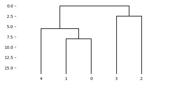
You can also plot a tree as dendrogram.
fig, ax = plt.subplots(figsize=(6.0, 6.0))
graphics.plot_dendrogram(ax, tree, labels=fruits)
fig.tight_layout()

From distances to trees
When you want to create a Tree from distances obtained for
example from sequence alignments, you can use the UPGMA or
neighbour joining algorithm.
distances = np.array([
    [ 0, 17, 21, 31, 23],
    [17, 0,  30, 34, 21],
    [21, 30, 0,  28, 39],
    [31, 34, 28,  0, 43],
    [23, 21, 39, 43,  0]
])
tree = phylo.upgma(distances)
fig, ax = plt.subplots(figsize=(6.0, 3.0))
graphics.plot_dendrogram(ax, tree, orientation="top")
fig.tight_layout()
Going 3D - The Structure subpackage
biotite.structure is a Biotite subpackage for handling
molecular structures.
This subpackage enables efficient and easy handling of protein structure
data by representing atom attributes in NumPy ndarray
objects.
These atom attributes include so called annotations
(polypetide chain id, residue id, residue name, hetero residue
information, atom name, element, etc.)
and the atom coordinates.
The package contains three central types: Atom,
AtomArray and AtomArrayStack.
An Atom contains data for a single atom, an AtomArray
stores data for an entire model and AtomArrayStack stores data
for multiple models, where each model contains the same atoms but
differs in the atom coordinates.
Both, AtomArray and AtomArrayStack, store the
attributes in NumPy arrays. This approach has multiple advantages:
Convenient selection of atoms in a structure by using NumPy style indexing
Fast calculations on structures using C-accelerated
ndarrayoperationsSimple implementation of custom calculations
Based on the implementation using ndarray objects, this package
also contains functions for structure analysis and manipulation.
Note
The universal length unit in Biotite is Å. This includes coordinates, distances, surface areas, etc.
Creating structures
Let’s begin by constructing some atoms:
import biotite.structure as struc

atom1 = struc.Atom([0,0,0], chain_id="A", res_id=1, res_name="GLY",
                   atom_name="N", element="N")
atom2 = struc.Atom([0,1,1], chain_id="A", res_id=1, res_name="GLY",
                   atom_name="CA", element="C")
atom3 = struc.Atom([0,0,2], chain_id="A", res_id=1, res_name="GLY",
                   atom_name="C", element="C")
The first parameter are the coordinates (internally converted into an
ndarray), the other parameters are annotations.
The annotations shown in this example are mandatory:
The chain ID, residue ID, residue name, insertion code, atom name,
element and whether the atom is not in protein/nucleotide chain
(hetero).
If you miss one of these, they will get a default value.
The mandatory annotation categories are originated in ATOM and
HETATM records in the PDB format.
The description of each annotation can be viewed in the
API reference.
Additionally, you can specify an arbitrary amount of custom
annotations, like B-factors, charge, etc.
In most cases you won’t work with Atom instances and in even
fewer cases Atom instances are created as it is done in the
above example.
If you want to work with an entire molecular structure, containing an
arbitrary amount of atoms, you have to use so called atom arrays.
An atom array can be seen as an array of atom instances
(hence the name).
But instead of storing Atom instances in a list, an
AtomArray instance contains one ndarray for each
annotation and the coordinates.
In order to see this in action, we first have to create an array from
the atoms we constructed before.
Then we can access the annotations and coordinates of the atom array
simply by specifying the attribute.
import numpy as np

array = struc.array([atom1, atom2, atom3])
print("Chain ID:", array.chain_id)
print("Residue ID:", array.res_id)
print("Atom name:", array.atom_name)
print("Coordinates:", array.coord)
print()
print(array)
Chain ID: ['A' 'A' 'A']
Residue ID: [1 1 1]
Atom name: ['N' 'CA' 'C']
Coordinates: [[0. 0. 0.]
 [0. 1. 1.]
 [0. 0. 2.]]

    A       1  GLY N      N         0.000    0.000    0.000
    A       1  GLY CA     C         0.000    1.000    1.000
    A       1  GLY C      C         0.000    0.000    2.000
The array() builder function takes any iterable object
containing Atom instances.
If you wanted to, you could even use another AtomArray, which
functions also as an iterable object of Atom objects.
An alternative way of constructing an array would be creating an
AtomArray by using its constructor, which fills the
annotation arrays and coordinates with the type respective zero
value.
In our example all annotation arrays have a length of 3, since we used
3 atoms to create it.
A structure containing n atoms is represented by annotation arrays
of length n and coordinates of shape (n,3).
As the annotations and coordinates are simply ndarray
objects, they can be edited in the same manner.
array.chain_id[:] = "B"
array.coord[array.element == "C", 0] = 42
# It is also possible to replace an entire annotation with another array
array.res_id = np.array([1,2,3])
print(array)
B       1  GLY N      N         0.000    0.000    0.000
B       2  GLY CA     C        42.000    1.000    1.000
B       3  GLY C      C        42.000    0.000    2.000
Apart from the structure manipulation functions we see later on, this is the usual way to edit structures in Biotite.
Warning
For editing an annotation, the index must be applied to
the annotation and not to the AtomArray, e.g.
array.chain_id[...] = "B" instead of
array[...].chain_id = "B".
The latter example is incorrect, as it creates a subarray of the
initial AtomArray (discussed later) and then tries to
replace the annotation array with the new value.
If you want to add further annotation categories to an array, you have
to call the add_annotation() or set_annotation()
method at first. After that you can access the new annotation array
like any other annotation array.
array.add_annotation("foo", dtype=bool)
array.set_annotation("bar", [1, 2, 3])
print(array.foo)
print(array.bar)
[False False False]
[1 2 3]
In some cases, you might need to handle structures, where each atom is
present in multiple locations
(multiple models in NMR structures, MD trajectories).
For the cases AtomArrayStack objects are used, which
represent a list of atom arrays.
Since the atoms are the same for each frame, but only the coordinates
change, the annotation arrays in stacks are still the same length n
ndarray objects as in atom arrays.
However, a stack stores the coordinates in a (m,n,3)-shaped
ndarray, where m is the number of frames.
A stack is constructed with stack() analogous to the code
snipped above.
It is crucial that all arrays that should be stacked
have the same annotation arrays, otherwise an exception is raised.
For simplicity reasons, we create a stack containing two identical
models, derived from the previous example.
stack = struc.stack([array, array.copy()])
print(stack)
Model 1
    B       1  GLY N      N         0.000    0.000    0.000
    B       2  GLY CA     C        42.000    1.000    1.000
    B       3  GLY C      C        42.000    0.000    2.000

Model 2
    B       1  GLY N      N         0.000    0.000    0.000
    B       2  GLY CA     C        42.000    1.000    1.000
    B       3  GLY C      C        42.000    0.000    2.000
Loading structures from file
Reading PDB files
Usually structures are not built from scratch, but they are read from
a file.
Probably one of the most popular structure file formats to date is the
Protein Data Bank Exchange (PDB) format.
For our purpose, we will work on a protein structure as small as
possible, namely the miniprotein TC5b (PDB: 1L2Y).
The structure of this 20-residue protein (304 atoms) has been
elucidated via NMR.
Thus, the corresponding PDB file consists of multiple (namely 38)
models, each showing another conformation.
At first we load the structure from a PDB file via the class
PDBFile in the subpackage biotite.structure.io.pdb.
from tempfile import gettempdir, NamedTemporaryFile
import biotite.structure.io.pdb as pdb
import biotite.database.rcsb as rcsb

pdb_file_path = rcsb.fetch("1l2y", "pdb", gettempdir())
pdb_file = pdb.PDBFile.read(pdb_file_path)
tc5b = pdb_file.get_structure()
print(type(tc5b).__name__)
print(tc5b.stack_depth())
print(tc5b.array_length())
print(tc5b.shape)
AtomArrayStack
38
304
(38, 304)
The method PDBFile.get_structure() returns an atom array stack
unless the model parameter is specified,
even if the file contains only one model.
Alternatively, the module level function get_structure()
can be used.
The following example
shows how to write an atom array or stack back into a PDB file:
pdb_file = pdb.PDBFile()
pdb_file.set_structure(tc5b)
temp_file = NamedTemporaryFile(suffix=".pdb", delete=False)
pdb_file.write(temp_file.name)
temp_file.close()
Other information (authors, secondary structure, etc.) cannot be
easily from PDB files using PDBFile.
Working with the PDBx format
After all, the PDB format itself is deprecated now due to several
shortcomings and was replaced by the Protein Data Bank Exchange
(PDBx) format.
As PDBx has become the standard structure format, it is also the
format with the most comprehensive interface in Biotite.
Today, this format has two common encodings:
The original text-based Crystallographic Information Framework (CIF)
and the BinaryCIF format.
While the former is human-readable, the latter is more efficient in
terms of file size and parsing speed.
The biotite.structure.io.pdbx subpackage provides classes for
interacting with both formats, CIFFile and
BinaryCIFFile, respectively.
In the following section we will focus on CIFFile,
but BinaryCIFFile works analogous.
import biotite.structure.io.pdbx as pdbx

cif_file_path = rcsb.fetch("1l2y", "cif", gettempdir())
cif_file = pdbx.CIFFile.read(cif_file_path)
PDBx can be imagined as hierarchical dictionary, with several levels:
File: The entirety of the PDBx file.
Block: The data for a single structure (e.g. 1L2Y).
Category: A coherent group of data (e.g. atom_site describes the atoms). Each column in the category must have the same length
Column: Contains values of a specific type (e.g atom_site.Cartn_x contains the x coordinates for each atom). Contains two Data instances, one for the actual data and one for a mask. In a lot of categories a column contains only a single value.
Data: The actual data in form of a
ndarray.
Each level may contain multiple instances of the next lower level,
e.g. a category may contain multiple columns.
Each level is represented by a separate class, that ban be used like a
dictionary.
For CIF files these are CIFFile, CIFBlock,
CIFCategory, CIFColumn and CIFData.
Note that CIFColumn is not treated like a dictionary, but
instead has a data and mask attribute.
Now we can access the data like a dictionary of dictionaries.
block = cif_file["1L2Y"]
# If there is as single block, you can alternatively use `cif_file.block`
category = block["audit_author"]
column = category["name"]
data = column.data
print(data.array)
['Neidigh, J.W.' 'Fesinmeyer, R.M.' 'Andersen, N.H.']
The data access can be cut short, especially if a certain data type is expected instead of strings.
column = category["pdbx_ordinal"]
print(column.as_array(int))
[1 2 3]
As already mentioned, many categories contain only a single value per column. In this case it may be convenient to get only a single item instead of an array.
for key, column in block["citation"].items():
    print(f"{key:25}{column.as_item()}")
id                       primary
title                    Designing a 20-residue protein.
journal_abbrev           Nat.Struct.Biol.
journal_volume           9
page_first               425
page_last                430
year                     2002
journal_id_ASTM          NSBIEW
country                  US
journal_id_ISSN          1072-8368
journal_id_CSD           2024
book_publisher           ?
pdbx_database_id_PubMed  11979279
pdbx_database_id_DOI     10.1038/nsb798
Note the ? in the output.
It indicates that the value is masked as ‘unknown’.
That becomes clear when we look at the mask of that column.
mask = block["citation"]["book_publisher"].mask.array
print(mask)
print(pdbx.MaskValue(mask[0]))
[2]
MaskValue.MISSING
For setting/adding blocks, categories etc. we simply assign values as we would do with dictionaries.
category = pdbx.CIFCategory()
category["number"] = pdbx.CIFColumn(pdbx.CIFData([1, 2]))
category["person"] = pdbx.CIFColumn(pdbx.CIFData(["me", "you"]))
category["greeting"] = pdbx.CIFColumn(pdbx.CIFData(["Hi!", "Hello!"]))
block["greetings"] = category
print(category.serialize())
loop_
_greetings.number
_greetings.person
_greetings.greeting
1 me  Hi!
2 you Hello!
For the sake of brevity it is also possible to omit CIFColumn
and CIFData and even pass columns directly at category
creation.
category = pdbx.CIFCategory({
    # If the columns contain only a single value, no list is required
    "fruit": "apple",
    "color": "red",
    "taste": "delicious",
})
block["fruits"] = category
print(category.serialize())
_fruits.fruit   apple
_fruits.color   red
_fruits.taste   delicious
For BinaryCIFFile the usage is analogous.
bcif_file_path = rcsb.fetch("1l2y", "bcif", gettempdir())
bcif_file = pdbx.BinaryCIFFile.read(bcif_file_path)
for key, column in bcif_file["1L2Y"]["audit_author"].items():
    print(f"{key:25}{column.as_array()}")
name                     ['Neidigh, J.W.' 'Fesinmeyer, R.M.' 'Andersen, N.H.']
pdbx_ordinal             [1 2 3]
The main difference is that BinaryCIFData has an additional
encoding attribute that specifies how the data is encoded
in the binary representation.
A well chosen encoding can reduce the file size significantly.
# Default uncompressed encoding
array = np.arange(100)
print(pdbx.BinaryCIFData(array).serialize())
print("\nvs.\n")
# Delta encoding followed by run-length encoding
# [0, 1, 2, ...] -> [0, 1, 1, ...] -> [0, 1, 1, 99]
print(
    pdbx.BinaryCIFData(
        array,
        encoding = [
            # [0, 1, 2, ...] -> [0, 1, 1, ...]
            pdbx.DeltaEncoding(),
            # [0, 1, 1, ...] -> [0, 1, 1, 99]
            pdbx.RunLengthEncoding(),
            # [0, 1, 1, 99] -> b"\x00\x00..."
            pdbx.ByteArrayEncoding()
        ]
    ).serialize()
)
{'data': b'\x00\x00\x00\x00\x01\x00\x00\x00\x02\x00\x00\x00\x03\x00\x00\x00\x04\x00\x00\x00\x05\x00\x00\x00\x06\x00\x00\x00\x07\x00\x00\x00\x08\x00\x00\x00\t\x00\x00\x00\n\x00\x00\x00\x0b\x00\x00\x00\x0c\x00\x00\x00\r\x00\x00\x00\x0e\x00\x00\x00\x0f\x00\x00\x00\x10\x00\x00\x00\x11\x00\x00\x00\x12\x00\x00\x00\x13\x00\x00\x00\x14\x00\x00\x00\x15\x00\x00\x00\x16\x00\x00\x00\x17\x00\x00\x00\x18\x00\x00\x00\x19\x00\x00\x00\x1a\x00\x00\x00\x1b\x00\x00\x00\x1c\x00\x00\x00\x1d\x00\x00\x00\x1e\x00\x00\x00\x1f\x00\x00\x00 \x00\x00\x00!\x00\x00\x00"\x00\x00\x00#\x00\x00\x00$\x00\x00\x00%\x00\x00\x00&\x00\x00\x00\'\x00\x00\x00(\x00\x00\x00)\x00\x00\x00*\x00\x00\x00+\x00\x00\x00,\x00\x00\x00-\x00\x00\x00.\x00\x00\x00/\x00\x00\x000\x00\x00\x001\x00\x00\x002\x00\x00\x003\x00\x00\x004\x00\x00\x005\x00\x00\x006\x00\x00\x007\x00\x00\x008\x00\x00\x009\x00\x00\x00:\x00\x00\x00;\x00\x00\x00<\x00\x00\x00=\x00\x00\x00>\x00\x00\x00?\x00\x00\x00@\x00\x00\x00A\x00\x00\x00B\x00\x00\x00C\x00\x00\x00D\x00\x00\x00E\x00\x00\x00F\x00\x00\x00G\x00\x00\x00H\x00\x00\x00I\x00\x00\x00J\x00\x00\x00K\x00\x00\x00L\x00\x00\x00M\x00\x00\x00N\x00\x00\x00O\x00\x00\x00P\x00\x00\x00Q\x00\x00\x00R\x00\x00\x00S\x00\x00\x00T\x00\x00\x00U\x00\x00\x00V\x00\x00\x00W\x00\x00\x00X\x00\x00\x00Y\x00\x00\x00Z\x00\x00\x00[\x00\x00\x00\\\x00\x00\x00]\x00\x00\x00^\x00\x00\x00_\x00\x00\x00`\x00\x00\x00a\x00\x00\x00b\x00\x00\x00c\x00\x00\x00', 'encoding': [{'type': <TypeCode.INT32: 3>, 'kind': 'ByteArray'}]}

vs.

{'data': b'\x00\x00\x00\x00\x01\x00\x00\x00\x01\x00\x00\x00c\x00\x00\x00', 'encoding': [{'srcType': <TypeCode.INT32: 3>, 'origin': 0, 'kind': 'Delta'}, {'srcSize': 100, 'srcType': <TypeCode.INT32: 3>, 'kind': 'RunLength'}, {'type': <TypeCode.INT32: 3>, 'kind': 'ByteArray'}]}
While this low-level API is useful for using the entire potential of the PDBx format, most applications require only reading/writing a structure. As the BinaryCIF format is both, smaller and faster to parse, it is recommended to use it instead of the CIF format in Biotite.
tc5b = pdbx.get_structure(bcif_file)
# Do some fancy stuff
pdbx.set_structure(bcif_file, tc5b)
get_structure() creates automatically an
AtomArrayStack, even if the file actually contains only a
single model.
If you would like to have an AtomArray instead, you have to
specify the model parameter.
Reading trajectory files
If the package MDtraj is installed, Biotite provides a read/write
interface for different trajectory file formats.
All supported trajectory formats have in common, that they store
only coordinates.
These can be extracted as ndarray with the
get_coord() method.
from tempfile import NamedTemporaryFile
import requests
import biotite.structure.io.xtc as xtc

# Download 1L2Y as XTC file for demonstration purposes
temp_xtc_file = NamedTemporaryFile("wb", suffix=".xtc", delete=False)
response = requests.get(
    "https://raw.githubusercontent.com/biotite-dev/biotite/master/"
    "tests/structure/data/1l2y.xtc"
)
temp_xtc_file.write(response.content)

traj_file = xtc.XTCFile.read(temp_xtc_file.name)
coord = traj_file.get_coord()
print(coord.shape)
(38, 304, 3)
If only an excerpt of frames is desired, the behavior of the
read() function can be customized with the start, stop and
step parameters.
# Read only every second frame
traj_file = xtc.XTCFile.read(temp_xtc_file.name, step=2)
coord = traj_file.get_coord()
print(coord.shape)
(19, 304, 3)
In order to extract an entire structure, i.e. an
AtomArrayStack, from a trajectory file, a template
structure must be given, since the trajectory file contains only
coordinate information.
import biotite.database.rcsb as rcsb
import biotite.structure.io.pdbx as pdbx

pdbx_file = pdbx.BinaryCIFFile.read(rcsb.fetch("1l2y", "bcif", gettempdir()))
template = pdbx.get_structure(pdbx_file, model=1)

traj_file = xtc.XTCFile.read(temp_xtc_file.name)
trajectory = traj_file.get_structure(template)

temp_xtc_file.close()
Array indexing and filtering
Atom arrays and stacks can be indexed in a similar way a
ndarray is indexed.
In fact, the index is propagated to the coordinates and the annotation
arrays.
Therefore, all NumPy compatible types of indices can be used,
like boolean arrays, index arrays/lists, slices and, of course,
integer values.
Integer indices have a special role here, as they reduce the
dimensionality of the data type:
Indexing an AtomArrayStack with an integer results in an
AtomArray at the specified frame, indexing an AtomArray
with an integer yields the specified Atom.
Iterating over arrays and stacks reduces the dimensionality in an
analogous way.
Let’s demonstrate indexing with the help of the structure of TC5b.
from tempfile import gettempdir
import biotite.structure as struc
import biotite.database.rcsb as rcsb
import biotite.structure.io as strucio

file_path = rcsb.fetch("1l2y", "bcif", gettempdir())
stack = strucio.load_structure(file_path)
print(type(stack).__name__)
print(stack.shape)
# Get the third model
array = stack[2]
print(type(array).__name__)
print(array.shape)
# Get the fifth atom
atom = array[4]
print(type(atom).__name__)
print(atom.shape)
AtomArrayStack
(38, 304)
AtomArray
(304,)
Atom
()
load_structure() gives us an AtomArrayStack.
The first indexing step reduces the stack to an atom array and the
second indexing step reduces the array to a single atom.
The shape attribute gives the number of models and atoms, similarly
to the shape attribute of ndarray objects.
Alternatively, the stack_depth() or array_length()
methods can be used to get the number of models or atoms,
respectively.
The following code section shows some examples for how an atom array can be indexed.
# Get the first atom
atom = array[0]
# Get a subarray containing the first and third atom
subarray = array[[0,2]]
# Get a subarray containing a range of atoms using slices
subarray = array[100:200]
# Filter all carbon atoms in residue 1
subarray = array[(array.element == "C") & (array.res_id == 1)]
# Filter all atoms where the X-coordinate is smaller than 2
subarray = array[array.coord[:,0] < 2]
An atom array stack can be indexed in a similar way, with the difference, that the index specifies the frame(s).
# Get an atom array from the first model
subarray = stack[0]
# Get a substack containing the first 10 models
substack = stack[:10]
Stacks also have the speciality, that they can handle 2-dimensional indices, where the first dimension specifies the frame(s) and the second dimension specifies the atom(s).
# Get the first 100 atoms from the third model
subarray = stack[2, :100]
# Get the first 100 atoms from the models 3, 4 and 5
substack = stack[2:5, :100]
# Get the first atom in the second model
atom = stack[1,0]
# Get a stack containing arrays containing only the first atom
substack = stack[:, 0]
Furthermore, biotite.structure contains advanced filters,
that create boolean masks from an atom array using specific criteria.
Here is a small example.
backbone = array[struc.filter_peptide_backbone(array)]
print(backbone.atom_name)
['N' 'CA' 'C' 'N' 'CA' 'C' 'N' 'CA' 'C' 'N' 'CA' 'C' 'N' 'CA' 'C' 'N' 'CA'
 'C' 'N' 'CA' 'C' 'N' 'CA' 'C' 'N' 'CA' 'C' 'N' 'CA' 'C' 'N' 'CA' 'C' 'N'
 'CA' 'C' 'N' 'CA' 'C' 'N' 'CA' 'C' 'N' 'CA' 'C' 'N' 'CA' 'C' 'N' 'CA' 'C'
 'N' 'CA' 'C' 'N' 'CA' 'C' 'N' 'CA' 'C']
If you would like to know which atoms are in proximity to specific
coordinates, have a look at the CellList class.
Warning
For annotation editing Since AnnotatedSequence objects use base position
indices and Sequence objects use array position indices,
you will get different results for annot_seq[n:m].sequence and
annot_seq.sequence[n:m].
Representing bonds
Up to now we only looked into atom arrays whose atoms are merely
described by its coordinates and annotations.
But there is more: Chemical bonds can be described, too, using a
BondList!
Consider the following case: Your atom array contains four atoms:
N, CA, C and CB. CA is a central atom that is connected to
N, C and CB.
A BondList is created by passing a ndarray
containing pairs of integers, where each integer represents an index
in a corresponding atom array.
The pairs indicate which atoms share a bond.
Additionally, it is required to specify the number of atoms in the
atom array.
from tempfile import gettempdir
import biotite.structure as struc

array = struc.array([
    struc.Atom([0,0,0], atom_name="N"),
    struc.Atom([0,0,0], atom_name="CA"),
    struc.Atom([0,0,0], atom_name="C"),
    struc.Atom([0,0,0], atom_name="CB")
])
print("Atoms:", array.atom_name)
bond_list = struc.BondList(
    array.array_length(),
    np.array([[1,0], [1,2], [1,3]])
)
print("Bonds (indices):")
print(bond_list.as_array())
print("Bonds (atoms names):")
print(array.atom_name[bond_list.as_array()[:, :2]])
ca_bonds, ca_bond_types = bond_list.get_bonds(1)
print("Bonds of CA:", array.atom_name[ca_bonds])
Atoms: ['N' 'CA' 'C' 'CB']
Bonds (indices):
[[0 1 0]
 [1 2 0]
 [1 3 0]]
Bonds (atoms names):
[['N' 'CA']
 ['CA' 'C']
 ['CA' 'CB']]
Bonds of CA: ['N' 'C' 'CB']
When you look at the internal ndarray
(as given by BondList.as_array()), you see a third column
containing zeros.
This column describes each bond with values from the BondType
enum: 0 corresponds to BondType.ANY, which means that the type
of the bond is undefined.
This makes sense, since we did not define the bond types, when we
created the bond list.
The other thing that has changed is the index order:
Each bond is sorted so that the index with the lower index is the
first element.
Although a BondList uses a ndarray under the hood,
indexing works a little bit different:
The indexing operation is not applied to the internal
ndarray, instead it behaves like the same indexing operation
was applied to a corresponding atom array:
The bond list adjusts its indices so that they still point to the same
atoms as before.
Bonds that involve at least one atom, that has been removed, are
deleted as well.
We will try that by deleting the C atom.
mask = (array.atom_name != "C")
sub_array = array[mask]
sub_bond_list = bond_list[mask]
print("Atoms:", sub_array.atom_name)
print("Bonds (indices):")
print(sub_bond_list.as_array())
print("Bonds (atoms names):")
print(sub_array.atom_name[sub_bond_list.as_array()[:, :2]])
Atoms: ['N' 'CA' 'CB']
Bonds (indices):
[[0 1 0]
 [1 2 0]]
Bonds (atoms names):
[['N' 'CA']
 ['CA' 'CB']]
As you see, the the bonds involving the C (only a single one) are removed and the remaining indices are shifted.
Connecting atoms and bonds
We do not have to index the atom array and the bond list
separately.
For convenience reasons you can associate a BondList to an
AtomArray via the bonds attribute.
If no BondList is associated, bonds is None.
Every time the atom array is indexed, the index is also applied to the
associated bond list.
The same behavior applies to concatenations, by the way.
array.bonds = bond_list
sub_array = array[array.atom_name != "C"]
print("Bonds (atoms names):")
print(sub_array.atom_name[sub_array.bonds.as_array()[:, :2]])
Bonds (atoms names):
[['N' 'CA']
 ['CA' 'CB']]
Note, that some functionalities in Biotite even require that the
input structure has an associated BondList.
Reading and writing bonds
Up to now the bond information has been created manually, which is infeasible for larger molecules. Instead bond information can be loaded from and saved to some file formats, including PDBx and MOL files. We’ll try that on the structure of TC5b and look at the bond information of the third residue, a tyrosine.
import biotite.database.rcsb as rcsb
import biotite.structure.io.pdbx as pdbx

file_path = rcsb.fetch("1l2y", "bcif", gettempdir())
pdbx_file = pdbx.BinaryCIFFile.read(file_path)
# Essential: set the 'include_bonds' parameter to true
stack = pdbx.get_structure(pdbx_file, include_bonds=True)
tyrosine = stack[:, (stack.res_id == 3)]
print("Bonds (indices):")
print(tyrosine.bonds)
print("Bonds (atoms names):")
print(tyrosine.atom_name[tyrosine.bonds.as_array()[:, :2]])
Bonds (indices):
[[ 0  1  1]
 [ 0 12  1]
 [ 1  2  1]
 [ 1  4  1]
 [ 1 13  1]
 [ 2  3  2]
 [ 4  5  1]
 [ 4 14  1]
 [ 4 15  1]
 [ 5  6  6]
 [ 5  7  5]
 [ 6  8  5]
 [ 6 16  1]
 [ 7  9  6]
 [ 7 17  1]
 [ 8 10  6]
 [ 8 18  1]
 [ 9 10  5]
 [ 9 19  1]
 [10 11  1]
 [11 20  1]]
Bonds (atoms names):
[['N' 'CA']
 ['N' 'H']
 ['CA' 'C']
 ['CA' 'CB']
 ['CA' 'HA']
 ['C' 'O']
 ['CB' 'CG']
 ['CB' 'HB2']
 ['CB' 'HB3']
 ['CG' 'CD1']
 ['CG' 'CD2']
 ['CD1' 'CE1']
 ['CD1' 'HD1']
 ['CD2' 'CE2']
 ['CD2' 'HD2']
 ['CE1' 'CZ']
 ['CE1' 'HE1']
 ['CE2' 'CZ']
 ['CE2' 'HE2']
 ['CZ' 'OH']
 ['OH' 'HH']]
Not only the connected atoms, but also the the bond types are defined:
Here we have both, BondType.SINGLE and BondType.DOUBLE
bonds (1 and 2, respectively).
Bond information can also be automatically inferred from an
AtomArray or AtomArrayStack:
connect_via_residue_names() is able to connect atoms in
all residues that appear in the
Chemical Component Dictionary,
comprising every molecule that appears in any PDB entry.
In contrast, connect_via_distances() uses only distances
between atoms to infer the bonds.
However, this function creates only BondType.ANY bonds and might
connect wrong atoms in rare cases.
Since both functions have the mentioned limitations it is usually
better to read bond information directly from file, if available.
import biotite.structure.io.pdb as pdb

file_path = rcsb.fetch("1l2y", "pdb", gettempdir())
pdb_file = pdb.PDBFile.read(file_path)
stack = pdb_file.get_structure()
stack.bonds = struc.connect_via_residue_names(stack)
tyrosine = stack[:, (stack.res_id == 3)]
print("Bonds (indices):")
print(tyrosine.bonds)
print("Bonds (atoms names):")
print(tyrosine.atom_name[tyrosine.bonds.as_array()[:, :2]])
Bonds (indices):
[[ 0  1  1]
 [ 0 12  1]
 [ 1  2  1]
 [ 1  4  1]
 [ 1 13  1]
 [ 2  3  2]
 [ 4  5  1]
 [ 4 14  1]
 [ 4 15  1]
 [ 5  6  6]
 [ 5  7  5]
 [ 6  8  5]
 [ 6 16  1]
 [ 7  9  6]
 [ 7 17  1]
 [ 8 10  6]
 [ 8 18  1]
 [ 9 10  5]
 [ 9 19  1]
 [10 11  1]
 [11 20  1]]
Bonds (atoms names):
[['N' 'CA']
 ['N' 'H']
 ['CA' 'C']
 ['CA' 'CB']
 ['CA' 'HA']
 ['C' 'O']
 ['CB' 'CG']
 ['CB' 'HB2']
 ['CB' 'HB3']
 ['CG' 'CD1']
 ['CG' 'CD2']
 ['CD1' 'CE1']
 ['CD1' 'HD1']
 ['CD2' 'CE2']
 ['CD2' 'HD2']
 ['CE1' 'CZ']
 ['CE1' 'HE1']
 ['CE2' 'CZ']
 ['CE2' 'HE2']
 ['CZ' 'OH']
 ['OH' 'HH']]
Simulation boxes and unit cells
Depending on the source of the macromolecular structure, there might
be an associated unit cell or simulation box.
In this package such boxes are represented by (3,3)-shaped
ndarray objects, where each element in the array is one of
the three vectors spanning the box or unit cell.
Let’s create an orthorhombic box from the vector lengths and the
angles between the vectors.
from tempfile import gettempdir
import numpy as np
import biotite.structure as struc

# The function uses angles in radians
box = struc.vectors_from_unitcell(10, 20, 30, np.pi/2, np.pi/2, np.pi/2)
print("Box:")
print(box)
print("Box volume:", struc.box_volume(box))
print("Is the box orthogonal?:", struc.is_orthogonal(box))
cell = struc.unitcell_from_vectors(box)
print("Cell:")
print(cell)
Box:
[[10.  0.  0.]
 [ 0. 20.  0.]
 [ 0.  0. 30.]]
Box volume: 6000.0
Is the box orthogonal?: True
Cell:
(10.0, 20.0, 30.0, 1.5707964, 1.5707964, 1.5707964)
An atom array can have an associated box, which is used in functions,
that consider periodic boundary conditions.
Atom array stacks require a (m,3,3)-shaped ndarray,
that contains the box vectors for each model.
The box is accessed via the box attribute, which is None by
default.
When loaded from a structure file, the box described in the file is
automatically used.
import biotite.database.rcsb as rcsb
import biotite.structure.io as strucio

array = struc.AtomArray(length=100)
print(array.box)
array.box = struc.vectors_from_unitcell(10, 20, 30, np.pi/2, np.pi/2, np.pi/2)
print(array.box)
file_path = rcsb.fetch("3o5r", "bcif", gettempdir())
array = strucio.load_structure(file_path)
print(array.box)
None
[[10.  0.  0.]
 [ 0. 20.  0.]
 [ 0.  0. 30.]]
[[42.051  0.     0.   ]
 [ 0.    54.784  0.   ]
 [ 0.     0.    56.816]]
When loading a trajectory from an MD simulation, the molecules are
often fragmented over the periodic boundary.
While a lot of analysis functions can handle such periodic boundary
conditions automatically, some require completed molecules.
In this case you should use remove_pbc().
array = struc.remove_pbc(array)
Structure manipulation
The most basic way to manipulate a structure is to edit the annotation arrays or coordinates directly.
from tempfile import gettempdir
import biotite.database.rcsb as rcsb
import biotite.structure as struc
import biotite.structure.io.pdbx as pdbx

pdbx_file = pdbx.BinaryCIFFile.read(rcsb.fetch("1l2y", "bcif", gettempdir()))
structure = pdbx.get_structure(pdbx_file, model=1)
print("Before:")
print(structure[structure.res_id == 1])
print()
structure.coord += 100
print("After:")
print(structure[structure.res_id == 1])
Before:
    A       1  ASN N      N        -8.901    4.127   -0.555
    A       1  ASN CA     C        -8.608    3.135   -1.618
    A       1  ASN C      C        -7.117    2.964   -1.897
    A       1  ASN O      O        -6.634    1.849   -1.758
    A       1  ASN CB     C        -9.437    3.396   -2.889
    A       1  ASN CG     C       -10.915    3.130   -2.611
    A       1  ASN OD1    O       -11.269    2.700   -1.524
    A       1  ASN ND2    N       -11.806    3.406   -3.543
    A       1  ASN H1     H        -8.330    3.957    0.261
    A       1  ASN H2     H        -8.740    5.068   -0.889
    A       1  ASN H3     H        -9.877    4.041   -0.293
    A       1  ASN HA     H        -8.930    2.162   -1.239
    A       1  ASN HB2    H        -9.310    4.417   -3.193
    A       1  ASN HB3    H        -9.108    2.719   -3.679
    A       1  ASN HD21   H       -11.572    3.791   -4.444
    A       1  ASN HD22   H       -12.757    3.183   -3.294

After:
    A       1  ASN N      N        91.099  104.127   99.445
    A       1  ASN CA     C        91.392  103.135   98.382
    A       1  ASN C      C        92.883  102.964   98.103
    A       1  ASN O      O        93.366  101.849   98.242
    A       1  ASN CB     C        90.563  103.396   97.111
    A       1  ASN CG     C        89.085  103.130   97.389
    A       1  ASN OD1    O        88.731  102.700   98.476
    A       1  ASN ND2    N        88.194  103.406   96.457
    A       1  ASN H1     H        91.670  103.957  100.261
    A       1  ASN H2     H        91.260  105.068   99.111
    A       1  ASN H3     H        90.123  104.041   99.707
    A       1  ASN HA     H        91.070  102.162   98.761
    A       1  ASN HB2    H        90.690  104.417   96.807
    A       1  ASN HB3    H        90.892  102.719   96.321
    A       1  ASN HD21   H        88.428  103.791   95.556
    A       1  ASN HD22   H        87.243  103.183   96.706
Biotite provides also some transformation functions, for example
rotate() for rotations about the x-, y- or z-axis.
structure = pdbx.get_structure(pdbx_file, model=1)
print("Before:")
print(structure[structure.res_id == 1])
print()
# Rotation about z-axis by 90 degrees
structure = struc.rotate(structure, [0, 0, np.deg2rad(90)])
print("After:")
print(structure[structure.res_id == 1])
Before:
    A       1  ASN N      N        -8.901    4.127   -0.555
    A       1  ASN CA     C        -8.608    3.135   -1.618
    A       1  ASN C      C        -7.117    2.964   -1.897
    A       1  ASN O      O        -6.634    1.849   -1.758
    A       1  ASN CB     C        -9.437    3.396   -2.889
    A       1  ASN CG     C       -10.915    3.130   -2.611
    A       1  ASN OD1    O       -11.269    2.700   -1.524
    A       1  ASN ND2    N       -11.806    3.406   -3.543
    A       1  ASN H1     H        -8.330    3.957    0.261
    A       1  ASN H2     H        -8.740    5.068   -0.889
    A       1  ASN H3     H        -9.877    4.041   -0.293
    A       1  ASN HA     H        -8.930    2.162   -1.239
    A       1  ASN HB2    H        -9.310    4.417   -3.193
    A       1  ASN HB3    H        -9.108    2.719   -3.679
    A       1  ASN HD21   H       -11.572    3.791   -4.444
    A       1  ASN HD22   H       -12.757    3.183   -3.294

After:
    A       1  ASN N      N        -4.127   -8.901   -0.555
    A       1  ASN CA     C        -3.135   -8.608   -1.618
    A       1  ASN C      C        -2.964   -7.117   -1.897
    A       1  ASN O      O        -1.849   -6.634   -1.758
    A       1  ASN CB     C        -3.396   -9.437   -2.889
    A       1  ASN CG     C        -3.130  -10.915   -2.611
    A       1  ASN OD1    O        -2.700  -11.269   -1.524
    A       1  ASN ND2    N        -3.406  -11.806   -3.543
    A       1  ASN H1     H        -3.957   -8.330    0.261
    A       1  ASN H2     H        -5.068   -8.740   -0.889
    A       1  ASN H3     H        -4.041   -9.877   -0.293
    A       1  ASN HA     H        -2.162   -8.930   -1.239
    A       1  ASN HB2    H        -4.417   -9.310   -3.193
    A       1  ASN HB3    H        -2.719   -9.108   -3.679
    A       1  ASN HD21   H        -3.791  -11.572   -4.444
    A       1  ASN HD22   H        -3.183  -12.757   -3.294
For a complete list of transformation functions have a look in the API reference.
Structure analysis
This package would be almost useless, if there wasn’t some means to analyze your structures. Therefore, Biotite offers a bunch of functions for this purpose, reaching from simple bond angle and length measurements to more complex characteristics, like accessible surface area and secondary structure. The following section will introduce you to some of these functions, which should be applied to that good old structure of TC5b.
The examples shown in this section are only a small glimpse into the structure analysis toolset. Have a look into the API reference for more information.
Geometry measures
Let’s start with measuring some simple geometric characteristics, for example atom distances of CA atoms.
from tempfile import gettempdir
import biotite.structure as struc
import biotite.structure.io as strucio
import biotite.database.rcsb as rcsb

file_path = rcsb.fetch("1l2y", "bcif", gettempdir())
stack = strucio.load_structure(file_path)
# Filter only CA atoms
stack = stack[:, stack.atom_name == "CA"]

# Calculate distance between first and second CA in first frame
array = stack[0]
print("Atom to atom:", struc.distance(array[0], array[1]))
# Calculate distance between the first atom
# and all other CA atoms in the array
print("Array to atom:")
array = stack[0]
print(struc.distance(array[0], array))
# Calculate pairwise distances between the CA atoms in the first frame
# and the CA atoms in the second frame
print("Array to array:")
print(struc.distance(stack[0], stack[1]))
# Calculate the distances between all CA atoms in the stack
# and the first CA atom in the first frame
# The resulting array is too large, therefore only the shape is printed
print("Stack to atom:")
print(struc.distance(stack, stack[0,0]).shape)
# And finally distances between two adjacent CA in the first frame
array = stack[0]
print("Adjacent CA distances")
print(struc.distance(array[:-1], array[1:]))
Atom to atom: 3.876399
Array to atom:
[ 0.         3.876399   5.5766597  5.038891   6.316409   8.766815
  9.908135  10.614817  12.890331  14.806679  13.5011635 16.87541
 18.723566  17.224289  19.111933  16.193     15.514756  12.377812
 10.445933  12.058967 ]
Array to array:
[3.4344199  0.37241507 0.22178602 0.10823133 0.15207201 0.17017055
 0.22572783 0.47650498 0.29493213 0.1548351  0.2832347  0.40683934
 0.1355508  0.3676874  0.46464393 0.57544243 0.33707416 0.25703317
 0.34762198 0.38818687]
Stack to atom:
(38, 20)
Adjacent CA distances
[3.876399  3.8605015 3.87147   3.8455799 3.8666048 3.8585181 3.8818028
 3.860987  3.8909183 3.8635552 3.8862703 3.8756127 3.8746684 3.8655493
 3.8662775 3.8776622 3.8603828 3.8582468 3.8642192]
Like some other functions in biotite.structure, we are able to
pick any combination of an atom, atom array or stack. Alternatively
ndarray objects containing the coordinates can be provided.
Furthermore, we can measure bond angles and dihedral angles.
# Calculate angle between first 3 CA atoms in first frame
# (in radians)
print("Angle:", struc.angle(array[0],array[1],array[2]))
# Calculate dihedral angle between first 4 CA atoms in first frame
# (in radians)
print("Dihedral angle:", struc.dihedral(array[0],array[1],array[2],array[4]))
Angle: 1.6098708
Dihedral angle: 1.4903792
Note
The distance(), angle() and
dihedral() functions all have their pair_...()
counterparts, that take an atom array (stack) and
pairs/triplets/quadruplets of atom indices, of which the
distance/angle should be calculated.
Both variants can be setup to consider periodic boundary conditions
by setting the box or periodic parameter, respectively.
In some cases one is interested in the dihedral angles of the peptide backbone, \(\phi\), \(\psi\) and \(\omega\). In the following code snippet we measure these angles and create a simple Ramachandran plot for the first frame of TC5b.
import matplotlib.pyplot as plt
import numpy as np

array = strucio.load_structure(file_path)[0]
phi, psi, omega = struc.dihedral_backbone(array)
plt.plot(phi * 360/(2*np.pi), psi * 360/(2*np.pi),
        marker="o", linestyle="None")
plt.xlim(-180,180)
plt.ylim(-180,180)
plt.xlabel("$\phi$")
plt.ylabel("$\psi$")
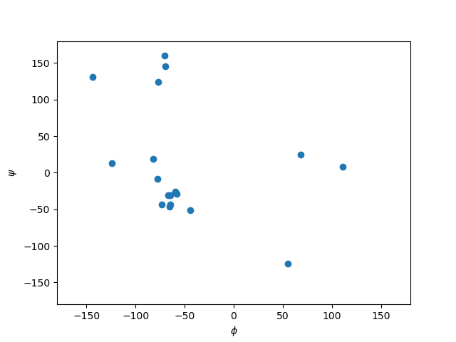
Text(26.472222222222214, 0.5, '$\\psi$')
Comparing structures
Now we want to calculate a measure of flexibility for each residue in TC5b. The root mean square fluctuation (RMSF) is a good value for that. It represents the deviation for each atom in all models relative to a reference model, which is usually the averaged structure. Since we are only interested in the backbone flexibility, we consider only CA atoms. Before we can calculate a reasonable RMSF, we have to superimpose each model on a reference model (we choose the first model), which minimizes the root mean square deviation (RMSD).
stack = strucio.load_structure(file_path)
# We consider only CA atoms
stack = stack[:, stack.atom_name == "CA"]
# Superimposing all models of the structure onto the first model
stack, transformation = struc.superimpose(stack[0], stack)
print("RMSD for each model to first model:")
print(struc.rmsd(stack[0], stack))
# Calculate the RMSF relative to the average of all models
rmsf = struc.rmsf(struc.average(stack), stack)
# Plotting stuff
plt.plot(np.arange(1,21), rmsf)
plt.xlim(0,21)
plt.xticks(np.arange(1,21))
plt.xlabel("Residue")
plt.ylabel("RMSF")
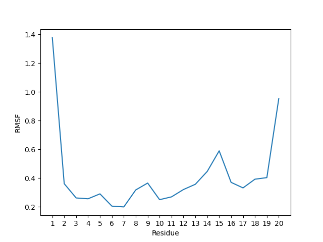
RMSD for each model to first model:
[0.         0.78426427 1.0075767  0.5518029  0.8066345  1.0606679
 0.87383705 0.6260642  1.0057654  0.81440794 0.87628293 1.353859
 0.93277997 0.8760094  0.99357307 0.4062658  0.3180194  1.1838905
 1.2347707  0.89114463 0.5553653  0.73639375 0.7856738  1.1019256
 0.6722887  1.1605636  0.9821395  1.2280883  0.79269636 0.868547
 0.9386667  0.835657   0.61650366 0.9733541  1.0322398  0.5555665
 1.1517521  0.8558534 ]

Text(42.597222222222214, 0.5, 'RMSF')
As you can see, both terminal residues are most flexible.
Calculating accessible surface area
Another interesting value for a protein structure is the
solvent accessible surface area (SASA) that indicates whether an
atom or residue is on the protein surface or buried inside the
protein.
The function sasa() approximates the SASA for each
atom.
Then we sum up the values for each residue, to get the
residue-wise SASA.
Besides other parameters, you can choose between different Van-der-Waals radii sets: Prot0r, the default set, is a set that defines radii for non-hydrogen atoms, but determines the radius of an atom based on the assumed amount of hydrogen atoms connected to it. Therefore, ProtOr is suitable for structures with missing hydrogen atoms, like crystal structures. Since the structure of TC5b was elucidated via NMR, we can assign a radius to every single atom (including hydrogens), hence we use the Single set.
array = strucio.load_structure(file_path)[0]
# The following line calculates the atom-wise SASA of the atom array
atom_sasa = struc.sasa(array, vdw_radii="Single")
# Sum up SASA for each residue in atom array
res_sasa = struc.apply_residue_wise(array, atom_sasa, np.sum)
# Again plotting stuff
plt.plot(np.arange(1,21), res_sasa)
plt.xlim(0,21)
plt.xticks(np.arange(1,21))
plt.xlabel("Residue")
plt.ylabel("SASA")
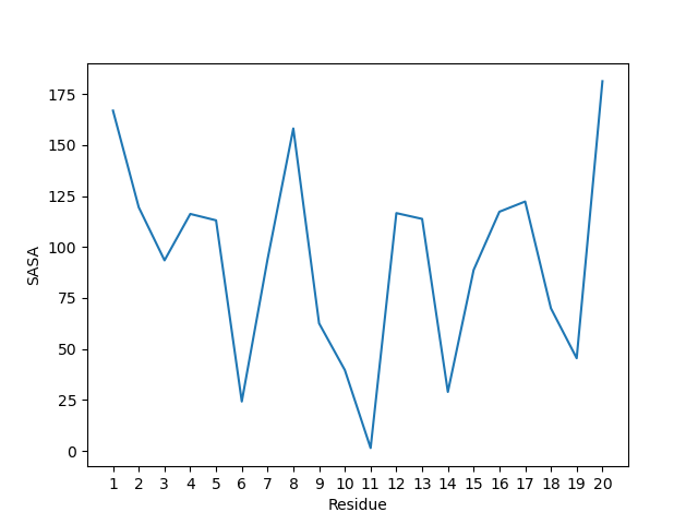
Text(38.097222222222214, 0.5, 'SASA')
Secondary structure determination
Biotite can also be used to assign
secondary structure elements (SSE) to a structure with the
annotate_sse() function.
An 'a' means alpha-helix, 'b' beta-sheet, and 'c' means
coil.
array = strucio.load_structure(file_path)[0]
# Estimate secondary structure
sse = struc.annotate_sse(array, chain_id="A")
# Pretty print
print("".join(sse))
caaaaaaaaccccccccccc
Outsourcing - The Application subpackage
Although you can achieve a lot with Biotite, there are still a lot of
things which are not implemented in this Python package.
But wait, this is what the biotite.application package is for:
It contains interfaces for popular external software.
This ranges from locally installed software to external tools running on
web servers.
The usage of these interfaces is seamless: Rather than writing input
files and reading output files, you simply put in your Python
objects (e.g. instances of Sequence or AtomArray) and
the interface returns Python objects (e.g. an Alignment
object).
Note
Note that in order to use an interface in
biotite.application the corresponding software must be
installed or the web server must be reachable, respectively.
These programs are not shipped with the Biotite package.
The base class for all interfaces is the Application class.
Each Application instance has a life cycle, starting with its
creation and ending with the result extraction.
Each state in this life cycle is described by the value of the
enum AppState, that each Application contains:
Directly after its instantiation the app is in the CREATED state.
In this state further parameters can be set for the application run.
After the user calls the Application.start() method, the app
state is set to RUNNING and the app performs the calculations.
When the application finishes the AppState
changes to FINISHED.
The user can now call the Application.join() method, concluding
the application in the JOINED state and making the results of the
application accessible.
Furthermore, this may trigger cleanup actions in some applications.
Application.join() can even be called in the RUNNING state:
This will constantly check if the application has finished and will
directly go into the JOINED state as soon as the application reaches
the FINISHED state.
Calling the Application.cancel() method while the application is
RUNNING or FINISHED leaves the application in the CANCELLED
state.
This triggers cleanup, too, but there are no accessible results.
If a method is called in an unsuitable app state, an
AppStateError is called.
At each state in the life cycle, Application type specific
methods are called, as shown in the following diagram.

The following sample code shows how an Application is generally
executed. Pay attention to the space between the
Application.start() and Application.join() method:
Since these are separate functions, you can do some other stuff, while
the Application runs in the background.
Thus, an Application behaves effectively like an additional
thread.
from biotite.application import Application

# Create a dummy Application subclass
class MyApplication(Application):
    def __init__(self, param): super().__init__()
    def run(self): pass
    def is_finished(self): return True
    def wait_interval(self): return 0.1
    def evaluate(self): pass
    def clean_up(self): pass
    def set_some_other_input(self, param): pass
    def get_some_data(self): return "some data"

param = "foo"
param2 = "bar"
app = MyApplication(param)
app.set_some_other_input(param2)
app.start()
# Time to do other stuff
app.join()
results = app.get_some_data()
The following subsections will dive into the available
Application classes in depth.
Finding homologous sequences with BLAST
the biotite.application.blast subpackage provides an
interface to NCBI BLAST: the BlastWebApp class.
Let’s dive directly into the code, we try to find
homologous sequences to the miniprotein TC5b:
import biotite.application.blast as blast
import biotite.sequence as seq

tc5b_seq = seq.ProteinSequence("NLYIQWLKDGGPSSGRPPPS")
app = blast.BlastWebApp("blastp", tc5b_seq)
app.start()
app.join()
alignments = app.get_alignments()
best_ali = alignments[0]
print(best_ali)
print()
print("HSP position in query: ", best_ali.query_interval)
print("HSP position in hit: ", best_ali.hit_interval)
print("Score: ", best_ali.score)
print("E-value: ", best_ali.e_value)
print("Hit UID: ", best_ali.hit_id)
print("Hit name: ", best_ali.hit_definition)
NLYIQWLKDGGPSSGRPPPS
NLYIQWLKDGGPSSGRPPPS

HSP position in query:  (1, 20)
HSP position in hit:  (1, 20)
Score:  101
E-value:  0.000161777
Hit UID:  1L2Y_A
Hit name:  Chain A, TC5b [synthetic construct]
This was too simple for BLAST:
As best hit it just found the query sequence itself in the PDB.
However, it gives a good impression about how this
Application works.
Besides some optional parameters, the BlastWebApp requires
the BLAST program and the query sequence. After the app has finished,
you get a list of alignments with descending score.
An alignment is an instance of BlastAlignment, a subclass of
biotite.sequence.align.Alignment.
It contains some additional information as shown above.
The hit UID can be used to obtain the complete hit sequence via
biotite.database.entrez.
The next alignment should be a bit more challenging. We take a random part of the E. coli BL21 genome and distort it a little bit. Since we still expect a high similarity to the original sequence, we decrease the E-value threshold.
import biotite.application.blast as blast
import biotite.sequence as seq

distorted_bl21_excerpt = seq.NucleotideSequence(
    "CGGAAGCGCTCGGTCTCCTGGCCTTATCAGCCACTGCGCGACGATATGCTCGTCCGTTTCGAAGA"
)
app = blast.BlastWebApp("blastn", distorted_bl21_excerpt, obey_rules=False)
app.set_max_expect_value(0.1)
app.start()
app.join()
alignments = app.get_alignments()
best_ali = alignments[0]
print(best_ali)
print()
print("HSP position in query: ", best_ali.query_interval)
print("HSP position in hit: ", best_ali.hit_interval)
print("Score: ", best_ali.score)
print("E-value: ", best_ali.e_value)
print("Hit UID: ", best_ali.hit_id)
print("Hit name: ", best_ali.hit_definition)
CGGAAGCGCTCGGTCTCCTGGCC---TTATCAGCCACTGCGCGACGATATGCTCGTCCGTTTCGAAGA
CGGAAGCGCT-GGTC-CCTGCCCGCTTTATCAGGGAATGCGCGACGGCAAAATCGTCCGTTTCGAAGA

HSP position in query:  (1, 65)
HSP position in hit:  (4656858, 4656923)
Score:  56
E-value:  0.0117615
Hit UID:  CP026845
Hit name:  Shigella boydii strain NCTC 9733 chromosome, complete genome
In this snippet we have set obey_rules to false in the
BlastWebApp constructor, if we omitted this parameter and
we started the last two code snippets in quick succession, a
RuleViolationError would be raised.
This is because normally the BlastWebApp respects NCBI’s code
of conduct and prevents you from submitting two queries within one
minute. If you want to be rude to the NCBI server, create the
instance with obey_rules set to false.
Multiple sequence alignments
For multiple sequence alignments (MSAs) biotite.application
offers several interfaces to MSA software.
For our example we choose the software MUSCLE:
The subpackage biotite.application.muscle contains the class
MuscleApp that does the job.
You simply input the sequences you want to have aligned, run the
application and get the resulting Alignment object.
import biotite.application.muscle as muscle
import biotite.sequence as seq

seq1 = seq.ProteinSequence("BIQTITE")
seq2 = seq.ProteinSequence("TITANITE")
seq3 = seq.ProteinSequence("BISMITE")
seq4 = seq.ProteinSequence("IQLITE")
app = muscle.MuscleApp([seq1, seq2, seq3, seq4])
app.start()
app.join()
alignment = app.get_alignment()
print(alignment)
BIQT-ITE
TITANITE
BISM-ITE
-IQL-ITE
In most MSA software even more information than the mere alignment can be extracted. For instance the guide tree, that was used for the alignment, can be obtained from the MUSCLE output.
import matplotlib.pyplot as plt
import biotite.sequence.graphics as graphics

tree = app.get_guide_tree()
fig, ax = plt.subplots()
graphics.plot_dendrogram(
    ax, tree, labels=[str(sequence) for sequence in [seq1, seq2, seq3, seq4]]
)
ax.set_xlabel("Distance")
fig.tight_layout()
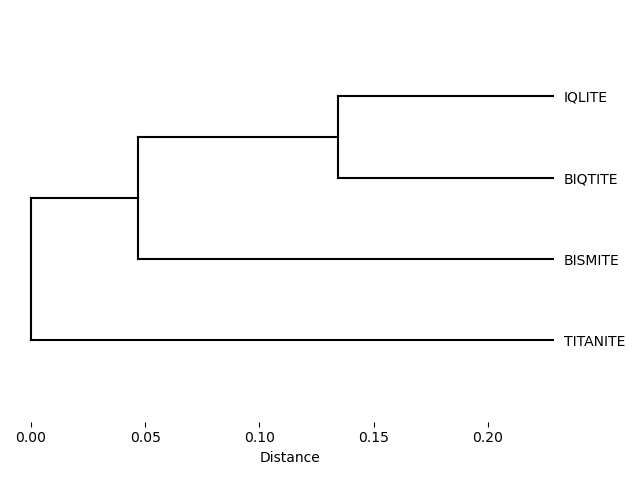
For the lazy people there is also a convenience method,
that handles the Application execution internally.
However, this shortcut returns only the Alignment.
alignment = muscle.MuscleApp.align([seq1, seq2, seq3, seq4])
The alternatives to MUSCLE are Clustal-Omega and MAFFT.
To use them, simply replace MuscleApp with
ClustalOmegaApp or MafftApp and you are done.
import biotite.application.clustalo as clustalo

alignment = clustalo.ClustalOmegaApp.align([seq1, seq2, seq3, seq4])
print(alignment)
-BIQTITE
TITANITE
-BISMITE
--IQLITE
As shown in the output, the alignment with Clustal-Omega slightly differs from the one performed with MUSCLE.
If the MSA software supports protein sequence alignment AND custom substitution matrices, e.g. MUSCLE and MAFFT, almost any type of sequence can be aligned: Internally the sequences and the matrix are converted into protein sequences/matrix. Then the masquerading sequences are aligned via the software and finally the sequences are mapped back into the original sequence type. Let’s show this on the example of a nonsense alphabet.
import numpy as np
import biotite.application.mafft as mafft
import biotite.sequence.align as align

alphabet = seq.Alphabet(("foo", "bar", 42))
sequences = [seq.GeneralSequence(alphabet, sequence) for sequence in [
    ["foo", "bar", 42, "foo", "foo", 42, 42],
    ["foo", 42, "foo", "bar", "foo", 42, 42],
]]
matrix = align.SubstitutionMatrix(
    alphabet, alphabet, np.array([
        [ 100, -100, -100],
        [-100,  100, -100],
        [-100, -100,  100]
    ])
)
alignment = mafft.MafftApp.align(sequences, matrix=matrix)
# As the alphabet do not has characters as symbols
# the alignment cannot be directly printed
# However, we can print the trace
print(alignment.trace)
[[ 0  0]
 [ 1 -1]
 [ 2  1]
 [ 3  2]
 [-1  3]
 [ 4  4]
 [ 5  5]
 [ 6  6]]
Secondary structure annotation
Althogh biotite.structure offers the function
annotate_sse() to assign secondary structure elements based on
the P-SEA algorithm, DSSP can also be used via the
biotite.application.dssp subpackage (provided that DSSP is
installed).
Let us demonstrate this on the example of the good old miniprotein
TC5b.
from tempfile import gettempdir
import biotite.database.rcsb as rcsb
import biotite.application.dssp as dssp
import biotite.structure.io as strucio

file_path = rcsb.fetch("1l2y", "bcif", gettempdir())
stack = strucio.load_structure(file_path)
array = stack[0]
app = dssp.DsspApp(array)
app.start()
app.join()
sse = app.get_sse()
print(sse)
['C' 'H' 'H' 'H' 'H' 'H' 'H' 'H' 'T' 'T' 'G' 'G' 'G' 'G' 'T' 'C' 'C' 'C'
 'C' 'C']
Similar to the MSA examples, DsspApp has the convenience
method DsspApp.annotate_sse() as shortcut.
