Comparative genome assembly of SARS-CoV-2 B.1.1.7 variant

In the following script we will perform a comparative genome assembly of the emerging SARS-CoV-2 B.1.1.7 variant in a simplified manner. We will use publicly available sequencing data of the virus variant produced from a Oxford Nanopore MinION and map these sequence snippets (reads) to the reference SARS-CoV-2 genome. Then we will create a single consensus sequence from the mapped reads and analyze where the differences to the reference genome are (variant calling). At last, we will focus on the mutations in the spike protein sequence.

Note

As the methods shown here are focused on simplicity, the accuracy of the assembled genome may be lower than the output from more sophisticated assembly software/pipelines.

To begin with, we download the relevant sequencing data from the NCBI sequence read archive (SRA) using Biotite’s interface to the SRA Toolkit. The software stores the downloaded sequence reads in one or multiple FASTQ files, one for each read per spot: A spot is a ‘location’ on the sequencing device. One spot may produce more than one read, e.g. Illumina sequencers use paired-end sequencing to produce a read starting from both ends of the original sequence. However, the MinION technology only creates one read per input sequence, so we expect only a single FASTQ file.

A FASTQ file provides for each read it contains

1. the sead sequence,

2. associated Phred quality scores.

Phred scores \(Q\) describe the accuracy of each base in the read in terms of base-call error probability \(P\) 1:

\[Q = -10 \log_{10} P\]

# Code source: Patrick Kunzmann
# License: BSD 3 clause

import itertools
import tempfile
from concurrent.futures import ProcessPoolExecutor
import numpy as np
import matplotlib.pyplot as plt
from matplotlib.lines import Line2D
from matplotlib.colors import LinearSegmentedColormap
import biotite
import biotite.sequence as seq
import biotite.sequence.align as align
import biotite.sequence.io as seqio
import biotite.sequence.io.fasta as fasta
import biotite.sequence.io.fastq as fastq
import biotite.sequence.io.genbank as gb
import biotite.sequence.graphics as graphics
import biotite.database.entrez as entrez
import biotite.application.sra as sra


# Download the sequencing data
app = sra.FastqDumpApp("SRR13453793")
app.start()
app.join()

# Load sequences and quality scores from the sequencing data
# There is only one read per spot
file_path = app.get_file_paths()[0]
fastq_file = fastq.FastqFile.read(file_path, offset="Sanger")
reads = [seq.NucleotideSequence(seq_str)
         for seq_str, score_array in fastq_file.values()]
score_arrays = [score_array for seq_str, score_array in fastq_file.values()]

print(f"Number of reads: {len(reads)}")

Number of reads: 58147

General sequencing data analysis

First we have a first glance on the quality of the sequencing data: the length of the reads and the Phred scores.

N_BINS = 200


fig, (length_ax, score_ax) = plt.subplots(nrows=2, figsize=(8.0, 6.0))

length_ax.hist(
    [len(score_array) for score_array in score_arrays],
    bins=np.logspace(1, 5, N_BINS), color="gray"
)
length_ax.set_xlabel("Read length")
length_ax.set_ylabel("Number of reads")
length_ax.set_xscale("log")
length_ax.set_yscale("log")

score_ax.hist(
    [np.mean(score_array) for score_array in score_arrays],
    bins=N_BINS, color="gray",
)
score_ax.set_xlim(0, 30)
score_ax.set_xlabel("Phred score")
score_ax.set_ylabel("Number of reads")

fig.tight_layout()

We can see the reads in the dataset are rather long, with most reads longer than 1 kb. This is one of the big advantages of the employed sequencing technology. Especially for de novo genome assembly (which we will not do here), long reads facilitate the process. However, the sequencing method also comes with a disadvantage: The base-call accuracy is relatively low, as the Phred scores indicate. Keep in mind, that \(Q = 10\) means that the called base at the respective position has a probability of 10 % to be wrong! Hence, a high sequencing depth, i.e. a large number of overlapping reads at each sequence position, is required to achieve accurate results. The partially low accuracy becomes even more visible, when creating a histogram over quality scores of individual bases, instead of averaging the scores over each read.

score_histogram = np.bincount(np.concatenate(score_arrays))

fig, ax = plt.subplots(figsize=(8.0, 4.0))
ax.fill_between(
    # Value in megabases -> 1e-6
    np.arange(len(score_histogram)), score_histogram * 1e-6,
    linewidth=0, color="gray"
)
ax.set_xlim(
    np.min(np.where(score_histogram > 0)[0]),
    np.max(np.where(score_histogram > 0)[0]),
)
ax.set_ylim(0, np.max(score_histogram * 1e-6) * 1.05)
ax.set_xlabel("Phred score")
ax.set_ylabel("Number of Mb")
fig.tight_layout()

Optionally, you could exclude or trim reads with exceptionally low Phred scores 2. But instead we rely on a high sequencing depth to filter out erroneous base calls.

Read mapping

In the next step we map each read to its respective position in the reference genome. An additional challenge is to find the correct sense of the read: In the library preparation both, sense and complementary DNA, is produced from the virus RNA. For this reason we need to create a complementary copy for each read and map both strands to the reference genome. Later the wrong strand is discarded.

# Download and read the reference SARS-CoV-2 genome
orig_genome_file = entrez.fetch(
    "NC_045512", tempfile.gettempdir(), "gb",
    db_name="Nucleotide", ret_type="gb"
)
orig_genome = seqio.load_sequence(orig_genome_file)

# Create complementary reads
compl_reads = list(itertools.chain(
    *[(read, read.reverse(False).complement()) for read in reads]
))

To map the reads to their corresponding positions in the reference genome, we need to align them to it. Although we could use align_optimal() (Needleman-Wunsch algorithm 3) for this purpose, aligning this large number of reads to even a small virus genome would take hours.

Instead we choose an heuristic alignment approach, similar to the method used by software like BLAST 4: First we scan each read for k-mer matches with the reference genome. A k-mer match is a subsequence of length k that appears in both the read an the reference genome. If k is chosen sufficiently large, such matches most likely occur in homologous sequence regions. Then we can perform an alignment that is restricted to the region of a match.

The KmerTable class allows the fast k-mer match scanning by tabulation of all k-mer positions in the reference genome sequence.

K = 12

genome_table = align.KmerTable.from_sequences(K, [orig_genome])

all_matches = []
for i, read in enumerate(compl_reads):
    all_matches.append(genome_table.match(read))

# k-mer tables use quite a large amount of RAM
# and we do not need this object anymore
del genome_table

However, we can expect a lot of consecutive k-mer match positions for each read: For example, for \(k = 3\), the nucleotide ACATT compared to itself would give matches for the k-mers ACA, CAT and ATT. The respective match positions would be (0,0), (1,1) and (2,2). However, the diagonal \(D = j - i\), where i and j are positions in the first and second sequence respectively, is always the same in this case: It is 0. The same applies for the read mapping: For the homologous region between the read and the genome all matches should be approximately on the same diagonal. Small deviations may arise from deletions/insertions (indels). As long as no indel occurs, the match diagonal should always be the same. However, we can expect to have some unspecific k-mer matches, too. But the diagonal of unspecific matches differs significantly from the diagonal of the ‘correct’ matches. Therefore, we select the diagonal with the highest frequency as the ‘correct’ diagonal for each read.

# Pick the matches for the 6th read as example
INDEX = 5
matches = all_matches[INDEX]
read_length = len(compl_reads[INDEX])

# Find the correct diagonal for the example read
diagonals = matches[:,2] - matches[:,0]
diag, counts = np.unique(diagonals, return_counts=True)
correct_diagonal = diag[np.argmax(counts)]

# Visualize the matches and the correct diagonal
fig, ax = plt.subplots(figsize=(8.0, 8.0))
ax.scatter(
    matches[:,0], matches[:,2],
    s=4, marker="o", color=biotite.colors["dimorange"], label="Match"
)
ax.plot(
    [0, read_length], [correct_diagonal, read_length+correct_diagonal],
    linestyle=":", linewidth=1.0, color="black", label="Correct diagonal"
)
ax.set_xlim(0, read_length)
ax.set_xlabel("Read position")
ax.set_ylabel("Reference genome position")
ax.legend()
fig.tight_layout()


# Find the correct diagonal for all reads
correct_diagonals = [None] * len(all_matches)
for i, matches in enumerate(all_matches):
    diagonals = matches[:,2] - matches[:,0]
    unqiue_diag, counts = np.unique(diagonals, return_counts=True)
    if len(unqiue_diag) == 0:
        # If no match is found for this sequence, ignore this sequence
        continue
    correct_diagonals[i] = unqiue_diag[np.argmax(counts)]
del matches

As already outlined, we would like to limit the alignment search space to the matching diagonal of the read and the reference genome (including some buffer to account for indels) to reduce the computation time. Hence, we use align_banded() to align the sequences. This function aligns two sequences within a diagonal band, defined by a lower diagonal \(D_L\) and an upper diagonal \(D_U\) 5. Two symbols at position i and j can only be aligned to each other, if \(D_L \leq j - i \leq D_U\). This also means, that the algorithm does not find an alignment, where due to indels it would leave the defined band.

We can safely center the band at the correct diagonal we obtained in the previous step for each read, but how do we choose the maximum deviation from the center of the band, i.e. the maximum number of indels we allow in either direction?

Statistics may help us here. As mentioned above, the utilized sequencing technique is relatively error-prone. Hence, let’s assume that the number of true indels between the original SARS-CoV-2 and the B.1.1.7 variant can be ignored compared to the larger number of indels introduced by sequencing errors. The indel error rates are approximately known for the MinION 6: insertion rate \(p_i = 0.03\), deletion rate \(p_d = 0.05\). Based on these probabilities we can define a band that will most probably be broad enough to cover the number of appearing read indels 7. \(\sigma\) gives the standard deviation from the correct diagonal and can be calculated as

\[\sigma = \sqrt{4 N (p_i + p_d - p_i^2 - p_d^2)}\]

where \(N\) is the read length. We choose \(3 \sigma\) as the deviation from the center of the band, resulting in a \(< 0.3\%\) chance that the optimal alignment path would leave the band.

Although, the computation time is massively reduced by using align_banded(), the gapped alignment step is still the most time-consuming one. Therefore, we use multiprocessing to spread the task to multiple cores on multi-core architectures.

P_INDEL = 4 * (0.03 + 0.05 - 0.03**2 - 0.05**2)

matrix = align.SubstitutionMatrix.std_nucleotide_matrix()

def map_sequence(read, diag):
    deviation = int(3 * np.sqrt(len(read) * P_INDEL))
    if diag is None:
        return None
    else:
        return align.align_banded(
            read, orig_genome, matrix, gap_penalty=-10,
            band = (diag - deviation, diag + deviation),
            max_number = 1
        )[0]

# Each process can be quite memory consuming
# -> Cap to two processes to make it work on low-RAM commodity hardware
with ProcessPoolExecutor(max_workers=2) as executor:
    alignments = list(executor.map(
        map_sequence, compl_reads, correct_diagonals, chunksize=1000
    ))

Now we have to select for each read, whether the original or complementary strand is the one homologous to the reference genome. We simply select the one with the higher score.

for_alignments = [alignments[i] for i in range(0, len(alignments), 2)]
rev_alignments = [alignments[i] for i in range(1, len(alignments), 2)]

scores = np.stack((
    [ali.score if ali is not None else 0 for ali in for_alignments],
    [ali.score if ali is not None else 0 for ali in rev_alignments]
),axis=-1)

correct_sense = np.argmax(scores, axis=-1)
correct_alignments = [for_a if sense == 0 else rev_a for for_a, rev_a, sense
                      in zip(for_alignments, rev_alignments, correct_sense)]
# If we use a reverse complementary read,
# we also need to reverse the Phred score arrays
correct_score_arrays = [score if sense == 0 else score[::-1] for score, sense
                        in zip(score_arrays, correct_sense)]

Now we know for each read where its corresponding position on the reference genome is. The mapping is complete. Eventually, we visualize the mapping.

# Find genome positions for the starts and ends of all reads
starts = np.array(
    [ali.trace[ 0, 1] for ali in correct_alignments if ali is not None]
)
stops = np.array(
    [ali.trace[-1, 1] for ali in correct_alignments if ali is not None]
)
# For a nicer plot sort these by their start position
order = np.argsort(starts)
starts = starts[order]
stops = stops[order]

fig, ax = plt.subplots(figsize=(8.0, 12.0))
ax.barh(
    np.arange(len(starts)), left=starts, width=stops-starts, height=1,
    color=biotite.colors["dimgreen"], linewidth=0
)
ax.set_ylim(0, len(starts)+1)
ax.spines['top'].set_visible(False)
ax.spines['right'].set_visible(False)
ax.spines['left'].set_visible(False)
ax.tick_params(left=False, labelleft=False)
ax.set_xlabel("Sequence position")
ax.set_title("Read mappings to reference genome")
fig.tight_layout()

Variant calling

Variant calling is the process of identifying substitutions and indels in the sequencing data compared to a reference genome. Generally, this task is not necessarily straight-forward: For example, the sequencing data might originate from to a diploid genome, so there might be two variants for each position due to heterozygosity. In our case we analyze a virus genome, so we expect only a single variant, which makes the challenge much easier.

Sophisticated variant calling methods may take a lot of factors into account, e.g. expected GC content, error rates, etc., to tackle the problem of erroneous base calls from the sequencer. In this script we take a rather simple approach.

Considering a single sequence location on the genome, we are interested in finding the most probable base from the sequencing data, or in other words the base that is least the result of a sequencing error. For a symbol (base) \(s \in \{ A, C, G, T\}\) the probability \(P\) of having a genotype \(G \neq s\) dependent on all base calls \(c_i\) is proportional to the product of the error probabilities for each base call, because each base call is considered an independent event.

\[P(G \neq s | c_1, ... c_n) \propto \prod_{i: c_i = s} p(G \neq s | c_i)\]

The proportionality instead of equality applies here, as this formula ignores base calls where \(c_i \neq s\), because these cases do not have an impact on which base is most probable.

As we consider the base that is least the result of a sequencing error as most probable genotype, we need to find \(s_G\), where

\[s_G = {\arg\min}_s \left( \prod_{i: c_i = s} p(G \neq s | c_i) \right).\]

We can replace the base call error probability \(p(G \neq s | c_i)\), as it is given by the Phred score.

\[s_G = {\arg\min}_s \left( \prod_{i: c_i = s} 10^{-\frac{Q_i}{10}} \right)\]

To simplify this equation we can take the logarithm of the product on the right expression, as the logarithm is a monotonic function.

\[ \begin{align}\begin{aligned}s_G = {\arg\min}_s \left( \sum_{i: c_i = s} log_{10}\left(10^{-\frac{Q_i}{10}}\right) \right)\\s_G = {\arg\min}_s \left( \sum_{i: c_i = s} -\frac{Q_i}{10} \right)\\s_G = {\arg\min}_s \left( \sum_{i: c_i = s} -Q_i \right)\\s_G = {\arg\max}_s \left( \sum_{i: c_i = s} Q_i \right)\end{aligned}\end{align} \]

This means we have to find the symbol with the maximum sum of supporting Phred scores. This approach is quite intuitive: The more often a base has been called, weighted with the certainty of the sequencer, the more likely this base is truly at this position.

Note

For the sake of brevity possible insertions into the reference genome are not considered in the method shown here.

# There are four possible bases for each genome position
phred_sum = np.zeros((len(orig_genome), 4), dtype=int)
# Track the sequencing depth over the genome for visualization purposes
sequencing_depth = np.zeros(len(orig_genome), dtype=int)
# Also track how many reads have called a deletion
# for each genome postion
deletion_number = np.zeros(len(orig_genome), dtype=int)

for alignment, score_array in zip(correct_alignments, correct_score_arrays):
    if alignment is not None:
        trace = alignment.trace

        no_gap_trace = trace[(trace[:,0] != -1) & (trace[:,1] != -1)]
        # Get the sequence code for the aligned read symbols
        seq_code = alignment.sequences[0].code[no_gap_trace[:,0]]
        # The sequence code contains the integers 0 - 3;
        # one for each possible base
        # Hence, we can use these integers directly to index the second
        # dimension of the Pred score sum
        # The index for the first dimension contains simply the genome
        # positions taken from the alignment trace
        phred_sum[no_gap_trace[:,1], seq_code] \
            += score_array[no_gap_trace[:,0]]

        sequencing_depth[
            trace[0,1] : trace[-1,1]
        ] += 1

        read_gap_trace = trace[trace[:,0] == -1]
        deletion_number[read_gap_trace[:,1]] += 1

# Call the most probable base for each genome position according to the
# formula above
most_probable_symbol_codes = np.argmax(phred_sum, axis=1)


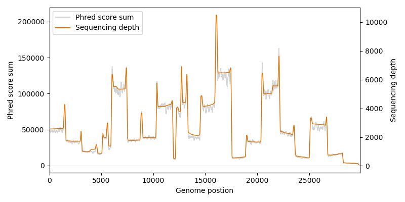
# Visualize the sequencing depth and score sum over the genome
max_phred_sum = phred_sum[
    np.arange(len(phred_sum)), most_probable_symbol_codes
]

def moving_average(data_set, window_size):
    weights = np.full(window_size, 1/window_size)
    return np.convolve(data_set, weights, mode='valid')

fig, ax = plt.subplots(figsize=(8.0, 4.0))
ax.plot(
    moving_average(max_phred_sum, 100),
    color="lightgray", linewidth=1.0
)
ax2 = ax.twinx()
ax2.plot(
    moving_average(sequencing_depth, 100),
    color=biotite.colors["dimorange"], linewidth=1.0
)
ax.axhline(0, color="silver", linewidth=0.5)
ax.set_xlim(0, len(orig_genome))
ax.set_xlabel("Genome postion")
ax.set_ylabel("Phred score sum")
ax2.set_ylabel("Sequencing depth")
ax.legend(
    [Line2D([0], [0], color=c)
     for c in ("lightgray", biotite.colors["dimorange"])],
    ["Phred score sum", "Sequencing depth"],
    loc="upper left"
)
fig.tight_layout()

We are finally reaching the last step of the assembly. Until now we only covered substitutions, but we also need to cover deletions. The statistics are more complex here, as a missing base in a read has of course no assigned Phred score. For the purpose of this example script we simply define as threshold: At least 60 % of all reads covering a certain location must call a deletion for this location, otherwise the deletion is rejected

DELETION_THRESHOLD = 0.6

var_genome = seq.NucleotideSequence()
var_genome.code = most_probable_symbol_codes
# A deletion is called, if either enough reads include this deletion
# or the sequence position is not covered by any read at all
deletion_mask = (deletion_number > sequencing_depth * DELETION_THRESHOLD) \
                | (sequencing_depth == 0)
var_genome = var_genome[~deletion_mask]
# Write the assembled genome into a FASTA file
out_file = fasta.FastaFile()
fasta.set_sequence(
    out_file, var_genome, header="SARS-CoV-2 B.1.1.7", as_rna=True
)
out_file.write(tempfile.NamedTemporaryFile("w"))

We have done it, the genome of the B.1.1.7 variant is assembled! Now we would like to have a closer look on the difference between the original and the B.1.1.7 genome.

Mutations in the B.1.1.7 variant

To get an rough overview about the overall sequence identity between the genomes and the locations of mutations in the B.1.1.7 variant, we need to align the original genome to our assembled one. As both genomes are expected to be highly similar, we can use a banded alignment again using a very conservative band width.

BAND_WIDTH = 1000

genome_alignment = align.align_banded(
    var_genome, orig_genome, matrix,
    band=(-BAND_WIDTH//2, BAND_WIDTH//2), max_number=1
)[0]
identity = align.get_sequence_identity(genome_alignment, 'all')
print(f"Sequence identity: {identity * 100:.2f} %")

Sequence identity: 99.76 %

Now we would like to have a closer look at the mutation locations. To contextualize the locations we plot the mutation frequency along with the gene locations. The genomic coordinates for each gene can be extracted from the already downloaded GenBank file of the reference genome.

N_BINS = 50

# Get genomic coordinates for all SARS-Cov-2 genes
gb_file = gb.GenBankFile.read(orig_genome_file)
annot_seq = gb.get_annotated_sequence(gb_file, include_only=["gene"])

# Calculate the sequence identity within each bin
bin_identities = np.zeros(N_BINS)
edges = np.linspace(0, len(orig_genome), N_BINS+1)
for i, (bin_start, bin_stop) in enumerate(zip(edges[:-1], edges[1:])):
    orig_genome_trace = genome_alignment.trace[:,1]
    excerpt = genome_alignment[
        (orig_genome_trace >= bin_start) & (orig_genome_trace < bin_stop)
    ]
    bin_identities[i] = align.get_sequence_identity(excerpt, "all")


fig, (deviation_ax, feature_ax) = plt.subplots(nrows=2, figsize=(8.0, 5.0))

# Plot the deviation = 1 - sequence identity
deviation_ax.bar(
    edges[:-1], width=(edges[1:]-edges[:-1]),
    height=(1 - bin_identities),
    color=biotite.colors["dimorange"], align="edge"
)
deviation_ax.set_xlim(0, len(orig_genome))
deviation_ax.set_ylabel("1 - Sequence identity")
deviation_ax.set_title("Sequence deviation of SARS-CoV-2 B.1.1.7 variant")
deviation_ax.set_yscale("log")
deviation_ax.set_ylim(1e-3, 1e-1)

# Plot genmic coordinates of the genes
for i, feature in enumerate(sorted(
    annot_seq.annotation,
    key=lambda feature: min([loc.first for loc in feature.locs])
)):
    for loc in feature.locs:
        feature_ax.barh(
            left=loc.first, width=loc.last-loc.first, y=i, height=1,
            color=biotite.colors["dimgreen"]
        )
        feature_ax.text(
            loc.last + 100, i, feature.qual["gene"],
            fontsize=8, ha="left", va="center"
        )
feature_ax.set_ylim(i+0.5, -0.5)
feature_ax.set_xlim(0, len(orig_genome))
feature_ax.xaxis.set_visible(False)
feature_ax.yaxis.set_visible(False)
feature_ax.set_frame_on(False)

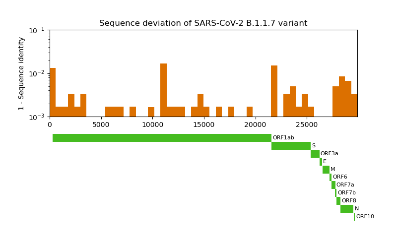
The S gene codes for the infamous spike protein: a membrane protein on the surface of SARS-CoV-2 that drives the infiltration of the host cell. Let’s have closer look on it.

Differences in the spike protein

For the investigation of the spike protein differences between the original and the variant SARS-CoV-2, we need to acquire the corresponding protein sequences. The location of the spike protein is annotated in the GenBank file for the reference genome. The homologous sequence for B.1.1.7 can be obtained by global sequence alignment of the spike gene sequence with the variant genome. Eventually, we can translate the gene sequences into protein sequences and compare them with each other - again by aligning them. To add meaning to the location of mutations we look at them in the context of the spike protein features/domains, which are well known 8.

SYMBOLS_PER_LINE = 75
SPACING = 3

# The locations of some notable spike protein regions
FEATURES = {
    # Signal peptide
    "SP":  (   1,   12),
    # N-terminal domain
    "NTD": (  14,  303),
    # Receptor binding domain
    "RBD": ( 319,  541),
    # Fusion peptide
    "FP":  ( 788,  806),
    # Transmembrane domain
    "TM":  (1214, 1234),
    # Cytoplasmatic tail
    "CT":  (1269, 1273),
}

# Get RNA sequence coding for spike protein from the reference genome
for feature in annot_seq.annotation:
    if feature.qual["gene"] == "S":
        orig_spike_seq = annot_seq[feature]

# Align spike protein sequence to variant genome to get the B.1.1.7
# spike protein sequence
alignment = align.align_optimal(
    var_genome, orig_spike_seq, matrix, local=True, max_number=1
)[0]
var_spike_seq = var_genome[alignment.trace[alignment.trace[:,0] != -1, 0]]

# Obtain protein sequences from RNA sequences
orig_spike_prot_seq = orig_spike_seq.translate(complete=True).remove_stops()
var_spike_prot_seq  =  var_spike_seq.translate(complete=True).remove_stops()

# Align both protein sequences with each other for later comparison
blosum_matrix = align.SubstitutionMatrix.std_protein_matrix()
alignment = align.align_optimal(
    var_spike_prot_seq, orig_spike_prot_seq, blosum_matrix, max_number=1
)[0]


fig = plt.figure(figsize=(8.0, 10.0))
ax = fig.add_subplot(111)

# Plot alignment
cmap = LinearSegmentedColormap.from_list(
    "custom", colors=[(1.0, 0.3, 0.3), (1.0, 1.0, 1.0)]
    #                    ^ reddish        ^ white
)
graphics.plot_alignment_similarity_based(
    ax, alignment, matrix=blosum_matrix, symbols_per_line=SYMBOLS_PER_LINE,
    labels=["B.1.1.7", "Reference"], show_numbers=True, label_size=9,
    number_size=9, symbol_size=7, spacing=SPACING, cmap=cmap
)

## Add indicator for features to the alignment
for row in range(1 + len(alignment) // SYMBOLS_PER_LINE):
    col_start = SYMBOLS_PER_LINE * row
    col_stop  = SYMBOLS_PER_LINE * (row + 1)
    if col_stop > len(alignment):
        # This happens in the last line
        col_stop = len(alignment)
    seq_start = alignment.trace[col_start, 1]
    seq_stop  = alignment.trace[col_stop-1,  1] + 1
    n_sequences = len(alignment.sequences)
    y_base = (n_sequences + SPACING) * row + n_sequences

    for feature_name, (first, last) in FEATURES.items():
        # Zero based sequence indexing
        start = first-1
        # Exclusive stop
        stop = last
        if start < seq_stop and stop > seq_start:
            # The feature is found in this line
            x_begin = np.clip(start - seq_start, 0, SYMBOLS_PER_LINE)
            x_end   = np.clip(stop - seq_start,  0, SYMBOLS_PER_LINE)
            x_mean = (x_begin + x_end) / 2
            y_line = y_base + 0.3
            y_text = y_base + 0.6
            ax.plot(
                [x_begin, x_end], [y_line, y_line],
                color="black", linewidth=2
            )
            ax.text(
                x_mean, y_text, feature_name,
                fontsize=8, va="top", ha="center"
            )
# Increase y-limit to include the feature indicators in the last line
ax.set_ylim(y_text, 0)
fig.tight_layout()

plt.show()

The most relevant mutations displayed here are the Δ69/70 deletion and the N501Y and D614G substitutions. Δ69/70 might allosterically change the protein conformation 9. D614G 10 and N501Y 11 increase the efficiency of host cell infection. For N501Y the reason is apparent: Being located in the RBD, this residue interacts directly with the human host cell receptor angiotensin-converting enzyme 2 (ACE2). Therefore, by increasing the binding affinity for ACE2, the infection is also facilitated.

References

1

P. J. A. Cock, C. J. Fields, N. Goto, M. L. Heuer, P. M. Rice, “The Sanger FASTQ file format for sequences with quality scores, and the Solexa/Illumina FASTQ variants,” Nucleic Acids Research, vol. 38, pp. 1767–1771, April 2010. doi: 10.1093/nar/gkp1137

2

S. Pabinger, A. Dander, M. Fischer, R. Snajder, M. Sperk, M. Efremova, B. Krabichler, M. R. Speicher, J. Zschocke, Z. Trajanoski, “A survey of tools for variant analysis of next-generation genome sequencing data,” Briefings in Bioinformatics, vol. 15, pp. 256–278, March 2014. doi: 10.1093/bib/bbs086

3

S. B. Needleman, C. D. Wunsch, “A general method applicable to the search for similarities in the amino acid sequence of two proteins,” Journal of Molecular Biology, vol. 48, pp. 443–453, March 1970. doi: 10.1016/0022-2836(70)90057-4

4

S. F. Altschul, W. Gish, W. Miller, E. W. Myers, D. J. Lipman, “Basic local alignment search tool,” Journal of Molecular Biology, vol. 215, pp. 403–410, October 1990. doi: 10.1016/S0022-2836(05)80360-2

5

K. Chao, W. R. Pearson, W. Miller, “Aligning two sequences within a specified diagonal band,” Bioinformatics, vol. 8, pp. 481–487, October 1992. doi: 10.1093/bioinformatics/8.5.481

6

A. D. Tyler, L. Mataseje, C. J. Urfano, L. Schmidt, K. S. Antonation, M. R. Mulvey, C. R. Corbett, “Evaluation of Oxford Nanopore’s MinION sequencing device for microbial whole genome sequencing applications,” Scientific Reports, vol. 8, pp. 10931, July 2018. doi: 10.1038/s41598-018-29334-5

7

J. Gibrat, “A short note on dynamic programming in a band,” BMC Bioinformatics, vol. 19, pp. 226, June 2018. doi: 10.1186/s12859-018-2228-9

8

X. Xia, “Domains and functions of spike protein in SARS-Cov-2 in the context of vaccine design,” Viruses, vol. 13, pp. 109, January 2021. doi: 10.3390/v13010109

9

X. Xie, Y. Liu, J. Liu, X. Zhang, J. Zou, C. R. {Fontes-Garfias}, H. Xia, K. A. Swanson, M. Cutler, D. Cooper, V. D. Menachery, S. C. Weaver, P. R. Dormitzer, P. Shi, “Neutralization of SARS-CoV-2 spike 69/70 deletion, E484K and N501Y variants by BNT162b2 vaccine-elicited sera,” Nature Medicine, pp. 1–2, February 2021. doi: 10.1038/s41591-021-01270-4

10

Z. Daniloski, T. X. Jordan, J. K. Ilmain, X. Guo, G. Bhabha, B. R. {tenOever}, N. E. Sanjana, “The Spike D614G mutation increases SARS-CoV-2 infection of multiple human cell types,” eLife, vol. 10, pp. e65365, February 2021. doi: 10.7554/eLife.65365

11

F. Tian, B. Tong, L. Sun, S. Shi, B. Zheng, Z. Wang, X. Dong, P. Zheng, “Mutation N501Y in RBD of spike protein strengthens the interaction between COVID-19 and its receptor ACE2,” bioRxiv, pp. 2021.02.14.431117, February 2021. doi: 10.1101/2021.02.14.431117