Three ways to get the secondary structure of a protein

In this example, we will obtain the secondary structure of the transketolase crystal structure (PDB: 1QGD) in three different ways and visualize it using a customized feature map.

At first, we will write draw functions for visualization of helices and sheets in feature maps.

# Code source: Patrick Kunzmann
# License: BSD 3 clause

from tempfile import gettempdir
import numpy as np
import matplotlib.pyplot as plt
from matplotlib.patches import Rectangle
import biotite
import biotite.structure as struc
import biotite.structure.io.pdbx as pdbx
import biotite.sequence as seq
import biotite.sequence.graphics as graphics
import biotite.sequence.io.genbank as gb
import biotite.database.rcsb as rcsb
import biotite.database.entrez as entrez
import biotite.application.dssp as dssp


# Create 'FeaturePlotter' subclasses
# for drawing the scondary structure features

class HelixPlotter(graphics.FeaturePlotter):

    def __init__(self):
        pass

    # Check whether this class is applicable for drawing a feature
    def matches(self, feature):
        if feature.key == "SecStr":
            if "sec_str_type" in feature.qual:
                if feature.qual["sec_str_type"] == "helix":
                    return True
        return False

    # The drawing function itself
    def draw(self, axes, feature, bbox, loc, style_param):
        # Approx. 1 turn per 3.6 residues to resemble natural helix
        n_turns = np.ceil((loc.last - loc.first + 1) / 3.6)
        x_val = np.linspace(0, n_turns * 2*np.pi, 100)
        # Curve ranges from 0.3 to 0.7
        y_val = (-0.4*np.sin(x_val) + 1) / 2

        # Transform values for correct location in feature map
        x_val *= bbox.width / (n_turns * 2*np.pi)
        x_val += bbox.x0
        y_val *= bbox.height
        y_val += bbox.y0

        # Draw white background to overlay the guiding line
        background = Rectangle(
            bbox.p0, bbox.width, bbox.height, color="white", linewidth=0
        )
        axes.add_patch(background)
        axes.plot(
            x_val, y_val, linewidth=2, color=biotite.colors["dimgreen"]
        )


class SheetPlotter(graphics.FeaturePlotter):

    def __init__(self, head_width=0.8, tail_width=0.5):
        self._head_width = head_width
        self._tail_width = tail_width


    def matches(self, feature):
        if feature.key == "SecStr":
            if "sec_str_type" in feature.qual:
                if feature.qual["sec_str_type"] == "sheet":
                    return True
        return False

    def draw(self, axes, feature, bbox, loc, style_param):
        x = bbox.x0
        y = bbox.y0 + bbox.height/2
        dx = bbox.width
        dy = 0

        if  loc.defect & seq.Location.Defect.MISS_RIGHT:
            # If the feature extends into the prevoius or next line
            # do not draw an arrow head
            draw_head = False
        else:
            draw_head = True

        axes.add_patch(biotite.AdaptiveFancyArrow(
            x, y, dx, dy,
            self._tail_width*bbox.height, self._head_width*bbox.height,
            # Create head with 90 degrees tip
            # -> head width/length ratio = 1/2
            head_ratio=0.5, draw_head=draw_head,
            color=biotite.colors["orange"], linewidth=0
        ))


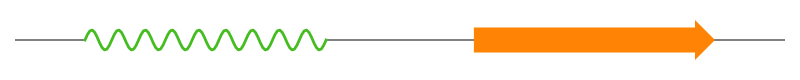
# Test our drawing functions with example annotation
annotation = seq.Annotation([
    seq.Feature("SecStr", [seq.Location(10, 40)], {"sec_str_type" : "helix"}),
    seq.Feature("SecStr", [seq.Location(60, 90)], {"sec_str_type" : "sheet"}),
])

fig = plt.figure(figsize=(8.0, 0.8))
ax = fig.add_subplot(111)
graphics.plot_feature_map(
    ax, annotation, multi_line=False, loc_range=(1,100),
    # Register our drawing functions
    feature_plotters=[HelixPlotter(), SheetPlotter()]
)
fig.tight_layout()

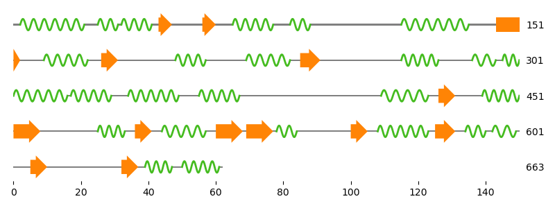
Now let us do some serious application. We want to visualize the secondary structure of one monomer of the homodimeric transketolase (PDB: 1QGD). The simplest way to do that, is to fetch the corresponding GenBank file, extract an Annotation object from the file and draw the annotation.

# Fetch GenBank files of the TK's first chain and extract annotatation
file_name = entrez.fetch("1QGD_A", gettempdir(), "gb", "protein", "gb")
gb_file = gb.GenBankFile.read(file_name)
annotation = gb.get_annotation(gb_file, include_only=["SecStr"])
# Length of the sequence
_, length, _, _, _, _ = gb.get_locus(gb_file)

fig = plt.figure(figsize=(8.0, 3.0))
ax = fig.add_subplot(111)
graphics.plot_feature_map(
    ax, annotation, symbols_per_line=150,
    show_numbers=True, show_line_position=True,
    # 'loc_range' takes exclusive stop -> length+1 is required
    loc_range=(1,length+1),
    feature_plotters=[HelixPlotter(), SheetPlotter()]
)
fig.tight_layout()

Next we calculate the secondary structure using the DSSP software from structure.

# Converter for the DSSP secondary structure elements
# to the classical ones
dssp_to_abc = {"I" : "c",
               "S" : "c",
               "H" : "a",
               "E" : "b",
               "G" : "c",
               "B" : "b",
               "T" : "c",
               "C" : "c"}

def visualize_secondary_structure(sse, first_id):
    """
    Helper function to convert secondary structure array to annotation
    and visualize it.
    """

    def _add_sec_str(annotation, first, last, str_type):
        if str_type == "a":
            str_type = "helix"
        elif str_type == "b":
            str_type = "sheet"
        else:
            # coil
            return
        feature = seq.Feature(
            "SecStr", [seq.Location(first, last)], {"sec_str_type" : str_type}
        )
        annotation.add_feature(feature)

    # Find the intervals for each secondary structure element
    # and add to annotation
    annotation = seq.Annotation()
    curr_sse = None
    curr_start = None
    for i in range(len(sse)):
        if curr_start is None:
            curr_start = i
            curr_sse = sse[i]
        else:
            if sse[i] != sse[i-1]:
                _add_sec_str(
                    annotation, curr_start+first_id, i-1+first_id, curr_sse
                )
                curr_start = i
                curr_sse = sse[i]
    # Add last secondary structure element to annotation
    _add_sec_str(annotation, curr_start+first_id, i-1+first_id, curr_sse)

    fig = plt.figure(figsize=(8.0, 3.0))
    ax = fig.add_subplot(111)
    graphics.plot_feature_map(
        ax, annotation, symbols_per_line=150,
        loc_range=(first_id, first_id+len(sse)),
        show_numbers=True, show_line_position=True,
        feature_plotters=[HelixPlotter(), SheetPlotter()]
    )
    fig.tight_layout()

# Fetch and load structure
file_name = rcsb.fetch("1QGD", "bcif", gettempdir())
pdbx_file = pdbx.BinaryCIFFile.read(file_name)
array = pdbx.get_structure(pdbx_file, model=1)
# Transketolase homodimer
tk_dimer = array[struc.filter_amino_acids(array)]
# Transketolase monomer
tk_mono = tk_dimer[tk_dimer.chain_id == "A"]

sse = dssp.DsspApp.annotate_sse(tk_mono)
sse = np.array([dssp_to_abc[e] for e in sse], dtype="U1")
visualize_secondary_structure(sse, tk_mono.res_id[0])

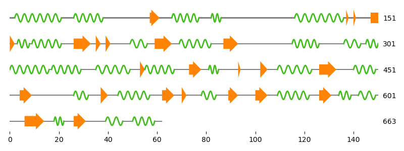
Last but not least we calculate the secondary structure using Biotite’s built-in method, based on the P-SEA algorithm.

sse = struc.annotate_sse(array, chain_id="A")
visualize_secondary_structure(sse, tk_mono.res_id[0])

plt.show()