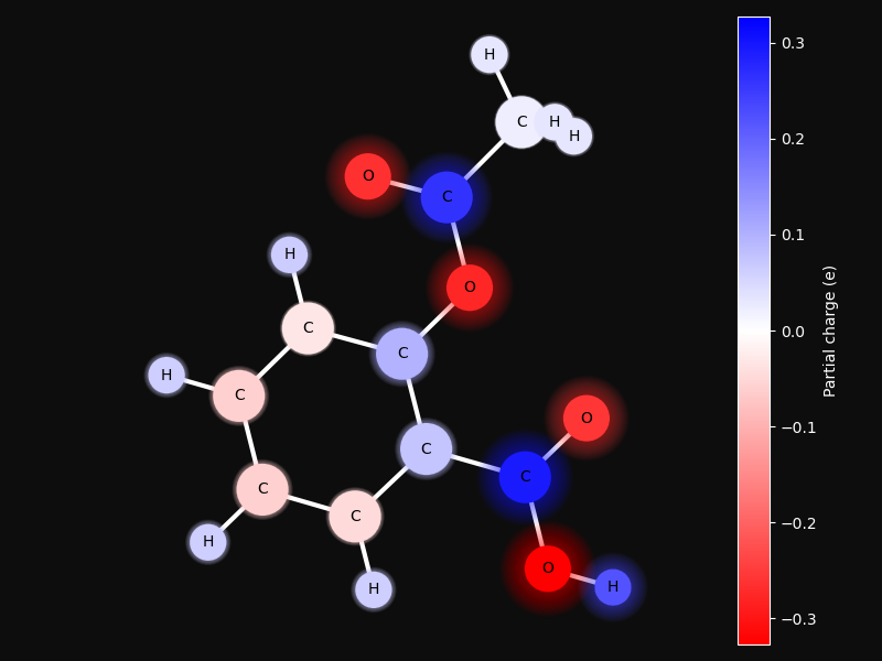
Partial charge distribution

This examples shows how partial charges are distributed in a small molecule. The charges are calculated using the PEOE method 1.

1

J. Gasteiger, M. Marsili, “Iterative partial equalization of orbital electronegativity—a rapid access to atomic charges,” Tetrahedron, vol. 36, pp. 3219–3228, January 1980. doi: 10.1016/0040-4020(80)80168-2

# Code source: Patrick Kunzmann
# License: BSD 3 clause

import numpy as np
from sklearn.decomposition import PCA
import matplotlib.pyplot as plt
from matplotlib.colors import Normalize
from matplotlib.cm import ScalarMappable
import biotite.structure as struc
import biotite.structure.info as info
import biotite.structure.graphics as graphics


# Acetylsalicylic acid
MOLECULE_NAME = "AIN"

# The number of iterations for the PEOE algorithm
ITERATION_NUMBER = 6
# The size of the element lables
ELEMENT_FONT_SIZE = 10
# The scaling factor of the atom 'balls'
BALL_SCALE = 20
# The higher this number, the more detailed are the rays
N_RAY_STEPS = 20
# The scaling factor of the 'ray' of charged molecules
RAY_SCALE = 100
# The transparency value for each 'ray ring'
RAY_ALPHA = 0.03
# The color map to use to depict the charge
CMAP_NAME = "bwr_r"



# Get an atom array for the selected molecule
molecule = info.residue(MOLECULE_NAME)

# Align molecule with principal component analysis:
# The component with the least variance, i.e. the axis with the lowest
# number of atoms lying over each other, is aligned to the z-axis,
# which points into the plane of the figure
pca = PCA(n_components=3)
pca.fit(molecule.coord)
molecule = struc.align_vectors(molecule, pca.components_[-1], [0, 0, 1])

# Balls should be colored by partial charge
charges = struc.partial_charges(molecule, ITERATION_NUMBER)
# Later this variable stores values between 0 and 1 for use in color map
normalized_charges = charges.copy()
# Show no partial charge for atoms
# that are not parametrized for the PEOE algorithm
normalized_charges[np.isnan(normalized_charges)] = 0
# Norm charge values to highest absolute value
max_charge = np.max(np.abs(normalized_charges))
normalized_charges /= max_charge
# Transform range (-1, 1) to range (0, 1)
normalized_charges = (normalized_charges + 1) / 2
# Calculate colors
color_map = plt.get_cmap(CMAP_NAME)
colors = color_map(normalized_charges)

# Ball size should be proportional to VdW radius of the respective atom
ball_sizes = np.array(
    [info.vdw_radius_single(e) for e in molecule.element]
) * BALL_SCALE

# Gradient of ray strength
# The ray size is proportional to the absolute charge value
ray_full_sizes = ball_sizes + np.abs(charges) * RAY_SCALE
ray_sizes = np.array([
    np.linspace(ray_full_sizes[i], ball_sizes[i], N_RAY_STEPS, endpoint=False)
    for i in range(molecule.array_length())
]).T


# The plotting begins here
fig = plt.figure(figsize=(8.0, 6.0))
ax = fig.add_subplot(111, projection="3d")

# Plot the atoms
# As 'axes.scatter()' uses sizes in points**2,
# the VdW-radii as also squared
graphics.plot_ball_and_stick_model(
    ax, molecule, colors, ball_size=ball_sizes**2, line_width=3,
    line_color=color_map(0.5), background_color=(.05, .05, .05), zoom=1.5
)

# Plot the element labels
for atom in molecule:
    ax.text(
        *atom.coord, atom.element,
        fontsize=ELEMENT_FONT_SIZE, color="black",
        ha="center", va="center", zorder=100
    )

# Plot the rays
for i in range(N_RAY_STEPS):
    ax.scatter(
        *molecule.coord.T, s=ray_sizes[i]**2, c=colors,
        linewidth=0, alpha=RAY_ALPHA
    )

# Plot the colorbar
color_bar = fig.colorbar(
    ScalarMappable(
        norm=Normalize(vmin=-max_charge, vmax=max_charge),
        cmap=color_map
    ),
    ax=ax
)
color_bar.set_label("Partial charge (e)", color="white")
color_bar.ax.yaxis.set_tick_params(color="white")
color_bar.outline.set_edgecolor("white")
for label in color_bar.ax.get_yticklabels():
    label.set_color("white")

fig.tight_layout()
plt.show()