Quality control of sequencing data

This script performs quality control on sequence reads similar to the FastQC software. This example is inspired by the Galaxy tutorial.

At first we fetch example sequencing data from the NCBI sequence read archive SRA. In this case we take data from whole genome sequencing of Escherichia virus phiX174. For the following script to work it is only important that each read has the exact same length.

# Code source: Patrick Kunzmann
# License: BSD 3 clause

import numpy as np
from scipy.stats import binom
import matplotlib.pyplot as plt
import matplotlib.ticker as ticker
import biotite
import biotite.sequence as seq
import biotite.application.sra as sra


FIG_SIZE = (8.0, 6.0)


app = sra.FastqDumpApp("ERR266411")
app.start()
app.join()
# Each run can have multiple reads per spot
# by selecting index 0 we take only the first read for every spot
sequences_and_scores = app.get_sequences_and_scores()[0]
sequence_codes = np.stack([
    sequence.code for sequence, _ in sequences_and_scores.values()
])
scores = np.stack([
    scores for _, scores in sequences_and_scores.values()
])
seq_count = scores.shape[0]
seq_length = scores.shape[1]
positions = np.arange(1, seq_length + 1)

We begin our analysis by investigating how the quality scores develop within the reads. Hence, we create something similar to a box plot for each read position. For the plot we need the first, second (the median) and third quartile for each position.

first_quartile, median, third_quartile = np.quantile(
    scores, (0.25, 0.5, 0.75), axis=0
)

fig, ax = plt.subplots(figsize=FIG_SIZE)
ax.bar(
    positions,
    bottom=first_quartile, height=third_quartile-first_quartile, width=1.0,
    facecolor=biotite.colors["brightorange"], label="Lower/upper quartile"
)
ax.plot(
    positions, median,
    color=biotite.colors["dimorange"], label="Median"
)
ax.set_xlim(positions[0], positions[-1])
ax.set_xlabel("Position in read")
ax.set_ylabel("Phred score")
ax.legend(loc="lower left")
fig.tight_layout()

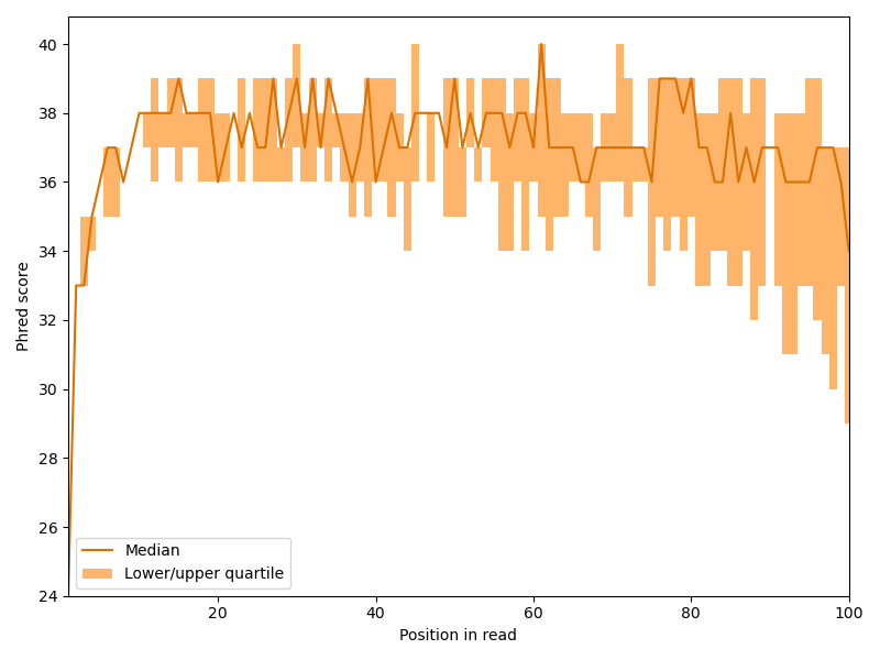
We can see that the Phred scores sharply increases the first few bases and then slowly drops with the length of the read, but overall, the quality is quite good. This behavior is quite common for Illumina sequencers.

Now we have a look at the other dimension: How is the quality distributed over the reads?

BIN_NUMBER = 500

mean_scores = np.mean(scores, axis=1)

fig, ax = plt.subplots(figsize=FIG_SIZE)
ax.hist(
    # Definition range of Sanger Phred scores is 0 to 40
    mean_scores, bins=np.linspace(0, 40, BIN_NUMBER),
    color=biotite.colors["lightorange"]
)
ax.set_xlabel("Mean Phred score of sequence")
ax.set_ylabel("Sequence count")
ax.set_xlim(
    np.floor(np.min(mean_scores)),
    np.ceil( np.max(mean_scores))
)
fig.tight_layout()

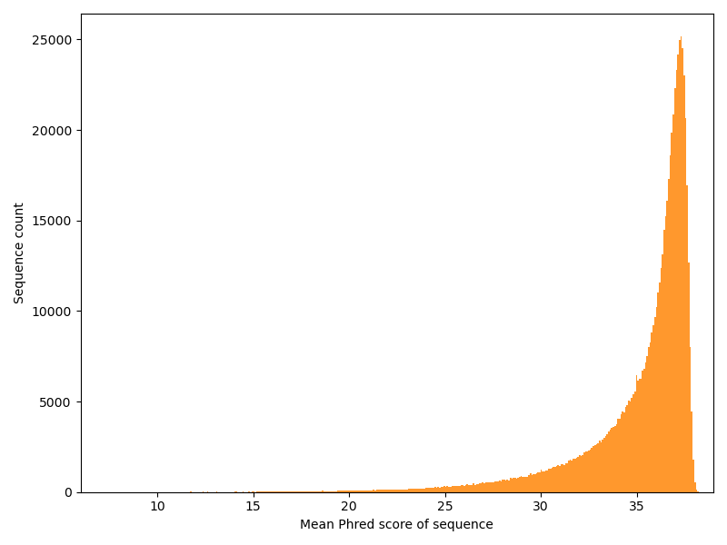
This is a typical distribution.

Now we want to see the appearance of each base over the length of the sequence reads. In a random library one would expect, that \(p(A) \approx p(T)\) and \(p(G) \approx p(C)\) for every position.

# Use ambiguous DNA alphabet,
# as ambiguous bases might occur in some sequencing datasets
alphabet = seq.NucleotideSequence.alphabet_amb

counts = np.stack([
    np.bincount(codes, minlength=len(alphabet))
    for codes in sequence_codes.T
], axis=-1)
frequencies = counts / seq_count * 100

fig, ax = plt.subplots(figsize=FIG_SIZE)
for character, freq in zip(alphabet.get_symbols(), frequencies):
    if (freq > 0).any():
        ax.plot(positions, freq, label=character)
ax.set_xlim(positions[0], positions[-1])
ax.xaxis.set_major_locator(ticker.AutoLocator())
ax.set_xlabel("Position in read")
ax.set_ylabel("Frequency at position (%)")
ax.legend(loc="upper left")
fig.tight_layout()

Again we have a look at the other dimension: How is the GC content distributed over the reads? If each position in all reads had a random base, we would expect a binomial distribution with a peak at the overall GC content. We plot our actual distribution along with the idealized binomial distribution.

gc_count = np.count_nonzero(
    (sequence_codes == alphabet.encode("G")) |
    (sequence_codes == alphabet.encode("C")),
    axis=1
)
at_count = np.count_nonzero(
    (sequence_codes == alphabet.encode("A")) |
    (sequence_codes == alphabet.encode("T")),
    axis=1
)
gc_content = gc_count / (gc_count + at_count)

# Exclusive range -> 0 to seq_length inclusive
number_of_gc = np.arange(seq_length+1)
exp_gc_content = binom.pmf(
    k=number_of_gc,
    n=seq_length,
    p=np.mean(gc_content)
)

fig, ax = plt.subplots(figsize=FIG_SIZE)
# Due to finite sequence length, the distribution is discrete
# -> use bar() instead of hist()
values, counts = np.unique(gc_content, return_counts=True)
bin_width = 100 / seq_length
ax.bar(
    values * 100, counts, width=bin_width,
    color=biotite.colors["brightorange"]
)
ax.plot(
    number_of_gc / seq_length * 100,
    exp_gc_content * seq_count,
    color=biotite.colors["dimorange"], linestyle=":"
)
ax.set_xlim(0, 100)
ax.set_xlabel("Sequence GC content (%)")
ax.set_ylabel("Sequence count")
fig.tight_layout()

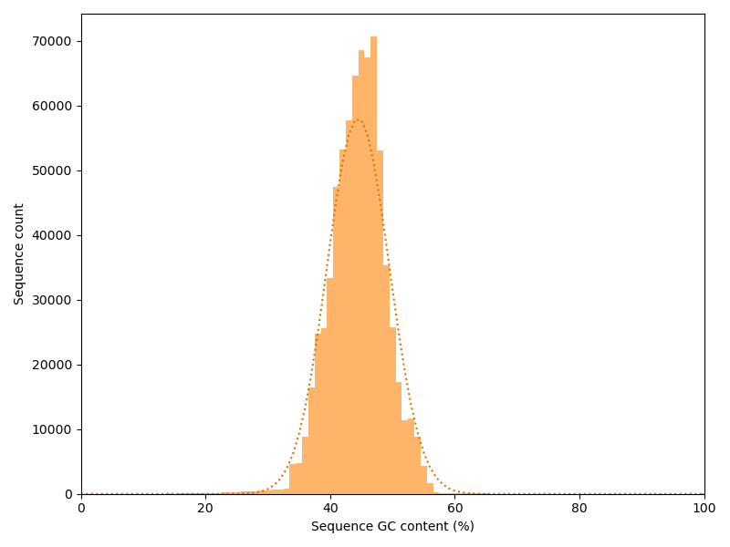
In this case the actual data stick relatively good to the idealized curve. Strong deviations may indicate contaminations or a biased library.

Finally, we investigate how often reads are duplicated in the dataset. For this purpose we create a dictionary that stores the sequences (or rather their sequence code) as keys and the number of duplications as values. Note that a duplication of number of 1 indicates that the sequence appears only once in the dataset.

duplications = {}
for code in sequence_codes:
    # NumPy arrays cannot be hashed -> convert array into tuple
    code = tuple(code)
    if code in duplications:
        duplications[code] += 1
    else:
        duplications[code] = 1
duplication_level_count = np.bincount(list(duplications.values()))
duplication_level_freq = (
    duplication_level_count
    * np.arange(len(duplication_level_count))
    / seq_count * 100
)
max_duplication = len(duplication_level_count)-1
print("Maximum duplication number:", max_duplication)

fig, ax = plt.subplots(figsize=FIG_SIZE)
ax.bar(
    np.arange(0, len(duplication_level_freq)),
    duplication_level_freq,
    width=0.6,
    color=biotite.colors["dimorange"]
)
ax.set_xlim(0.5, len(duplication_level_freq) + 0.5)
ax.xaxis.set_major_locator(ticker.MaxNLocator(10))
ax.set_xlabel("Number of duplications")
ax.set_ylabel("Sequence percentage (%)")
fig.tight_layout()

plt.show()

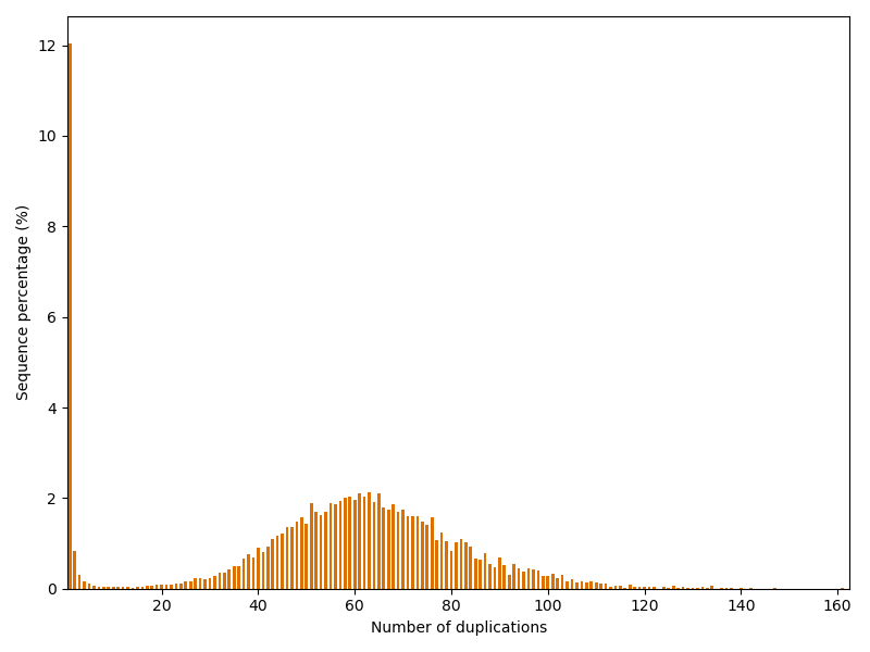
Maximum duplication number: 161

The dataset has quite an unusual repetition profile: Usually one would expect, that most sequences occur only once and the following duplication numbers become decreasingly likely. However, in this case we have another peak at around 60 duplications. And one read is even repeated astonishing 161 times!