Statistics of local alignments and the E-value

This example shows how to evaluate the significance of a local alignment of two sequences. The methods shown here are based on the approach presented by Altschul & Gish 1. The presented technique is also implemented in the EValueEstimator.

Let’s assume you have a query sequence (avidin) and you want to check, if there are homologous sequences in a hypothetical database. So you align the database sequences with your query sequence. Indeed, you found a sequence hit (streptavidin) in the database that looks quite similar to your sequence.

# Code source: Patrick Kunzmann
# License: BSD 3 clause

import matplotlib.pyplot as plt
from matplotlib.lines import Line2D
import numpy as np
from scipy.stats import linregress
import biotite
import biotite.sequence as seq
import biotite.sequence.align as align
from biotite.sequence.align.alignment import score
import biotite.sequence.io.fasta as fasta
import biotite.database.entrez as entrez
import biotite.sequence.graphics as graphics


GAP_PENALTY = (-12, -1)


# Download and parse protein sequences of avidin and streptavidin
fasta_file = fasta.FastaFile.read(entrez.fetch_single_file(
    ["CAC34569", "ACL82594"], None, "protein", "fasta"
))
for name, sequence in fasta_file.items():
    if "CAC34569" in name:
        query_seq = seq.ProteinSequence(sequence)
    elif "ACL82594" in name:
        hit_seq = seq.ProteinSequence(sequence)


# Get BLOSUM62 matrix
matrix = align.SubstitutionMatrix.std_protein_matrix()

# Perform pairwise sequence alignment with affine gap penalty
# Terminal gaps are not penalized
alignment = align.align_optimal(
    query_seq, hit_seq, matrix,
    local=True, gap_penalty=GAP_PENALTY, max_number=1
)[0]


print(f"Score: {alignment.score}")

fig = plt.figure(figsize=(8.0, 3.0))
ax = fig.add_subplot(111)
graphics.plot_alignment_similarity_based(
    ax, alignment, matrix=matrix, labels=["Avidin (query)", "Database hit"],
    show_numbers=True, show_line_position=True
)
fig.tight_layout()

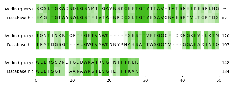
Score: 131

How can you make sure that you observe a true homology and not simply a product of coincidence? The value you have at hand is the similarity score of the alignment, but it is an absolute value that cannot be used without context to answer this question. But it can be used to ask another question: How many alignments with a score at least this high can you expect in this database by chance? We call this quantity expect value (E-value). If this value is close to 1 or even higher, we can assume that the reported alignment was found by chance. With decreasing E-value, the observed homology becomes more significant.

The remainder of this example will explain how to calculate the E-value for a given combination of query sequence, database size and scoring scheme.

The case of the ungapped local alignment

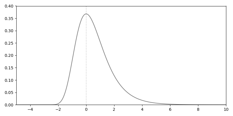
If no gaps can be inserted into an alignment, i.e. the gap penalty is infinite, the statistics can be solved analytically: The similarity score obtained by aligning two random sequences follows an extreme value distribution (\(f(x)\)), based on the two parameters \(u\) and \(\lambda\):

\[ \begin{align}\begin{aligned}t(x) = e^{-\lambda (x - u)}\\f(x) = \lambda t(x) e^{-t(x)}\end{aligned}\end{align} \]

# The probability density function of the extreme value distribution
def pdf(x, l, u):
    t = np.exp(-l * (x - u))
    return l * t * np.exp(-t)

x = np.linspace(-5, 10, 1000)
y = pdf(x, 1, 0)

fig, ax = plt.subplots(figsize=(8.0, 4.0))
ax.plot(x, y, color="gray", linestyle="-")
ax.axvline(0, color="silver", linestyle=":")
ax.set_xlim(-5, 10)
ax.set_ylim(0, 0.4)
fig.tight_layout()

\(u\) is calculated as

\[u = \frac{\ln Kmn}{\lambda},\]

where \(m\) and \(n\) are the lengths of the aligned sequences. \(K\) and \(\lambda\) can be calculated from the substitution matrix and the amino acid/nucleotide background frequencies. The probability to find an alignment with a score at least \(s\) becomes

\[P(S \geq s) = 1 - \exp(-Kmn e^{-\lambda s}).\]

This probability relates to the E-value with

\[P(S \geq s) = 1 - e^{-E}\]

resulting in a rather simple formula for the E-value:

\[E = Kmn e^{-\lambda s}\]

Estimating parameters for gapped alignments

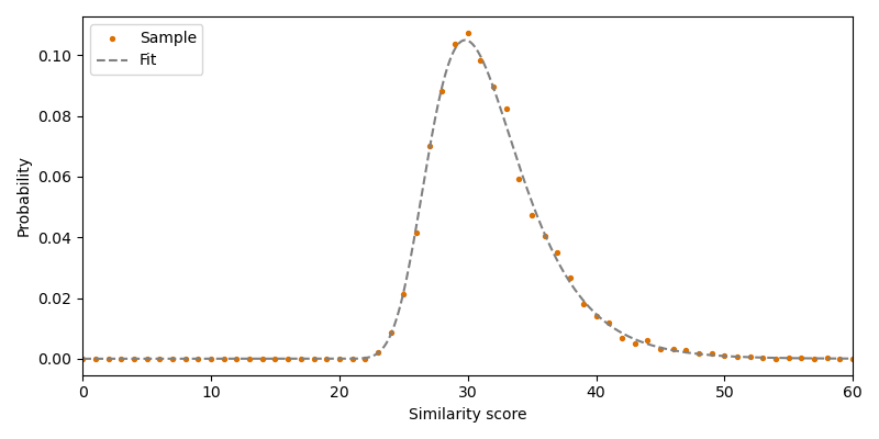
However, one usually handles alignments with gaps. Experiments show, that the extreme value distribution is also valid for gapped alignments. However the parameters \(u\) and \(\lambda\) need to be sampled. An easy way to achieve this, is to create a large number of pairs of sequences with representative background frequencies and fixed sequence length, align them and track the score. In this example we use a published set of amino acid frequencies 2, but the frequencies can be adjusted to represent the composition of the underlying sequence database.

SAMPLE_SIZE = 10000
SEQ_LENGTH = 300

BACKGROUND = np.array(list({
    "A": 35155,
    "C": 8669,
    "D": 24161,
    "E": 28354,
    "F": 17367,
    "G": 33229,
    "H": 9906,
    "I": 23161,
    "K": 25872,
    "L": 40625,
    "M": 10101,
    "N": 20212,
    "P": 23435,
    "Q": 19208,
    "R": 23105,
    "S": 32070,
    "T": 26311,
    "V": 29012,
    "W": 5990,
    "Y": 14488,
    "B": 0,
    "Z": 0,
    "X": 0,
    "*": 0,
}.values())) / 450431


# Generate the sequence code for random sequences
np.random.seed(0)
random_sequence_code = np.random.choice(
    np.arange(len(seq.ProteinSequence.alphabet)),
    size=(SAMPLE_SIZE, 2, SEQ_LENGTH),
    p=BACKGROUND
)

# Sample alignment scores
sample_scores = np.zeros(SAMPLE_SIZE, dtype=int)
for i in range(SAMPLE_SIZE):
    seq1 = seq.ProteinSequence()
    seq2 = seq.ProteinSequence()
    seq1.code = random_sequence_code[i,0]
    seq2.code = random_sequence_code[i,1]
    sample_alignment = align.align_optimal(
        seq1, seq2, matrix,
        local=True, gap_penalty=GAP_PENALTY, max_number=1
    )[0]
    sample_scores[i] = sample_alignment.score

There are multiple ways to estimate \(u\) and \(\lambda\) from the sampled similarity scores. Here we use the method of moments 3:

\[ \begin{align}\begin{aligned}\lambda = \frac{\pi}{\sqrt{6V}}\\u = \mu - \frac{\gamma}{\lambda}\end{aligned}\end{align} \]

where \(\gamma\) is Euler’s constant and \(\mu\) and \(V\) are the distribution mean and variance of the sampled scores, respectively.

# Use method of moments to estimate distribution parameters
l = np.pi / np.sqrt(6 * np.var(sample_scores))
u = np.mean(sample_scores) - np.euler_gamma / l

# Score frequencies for the histogram
freqs = np.bincount(sample_scores) / SAMPLE_SIZE

# Coordinates for the fit
x = np.linspace(0, len(freqs)-1, 1000)
y = pdf(x, l, u)

fig, ax = plt.subplots(figsize=(8.0, 4.0))
ax.scatter(
    np.arange(len(freqs)), freqs, color=biotite.colors["dimorange"],
    label="Sample", s=8
)
ax.plot(x, y, color="gray", linestyle="--", label="Fit")
ax.set_xlabel("Similarity score")
ax.set_ylabel("Probability")
ax.set_xlim(0, len(freqs)-1)
ax.legend(loc="upper left")
fig.tight_layout()

Generalization to arbitrary sequence lengths

This estimation would allow the calculation of the E-value for sequences with the employed lengths. However, for a query sequence of any other length you would need to conduct this time-costly calculation again.

Hence, let us check if the equation

\[u = \frac{\ln Kmn}{\lambda}\]

also holds for gapped alignments. If this is the case, we would expect a linear relation between \(u\) and \(\ln mn\), since

\[u = \ln K / \lambda + \frac{1}{\lambda} \ln mn\]

LENGTH_RANGE = (10, 2000)
LENGTH_SAMPLE_SIZE = 20
SAMPLE_SIZE_PER_LENGTH = 1000

# The sequence lengths to be sampled
length_samples = np.logspace(*np.log10(LENGTH_RANGE), LENGTH_SAMPLE_SIZE) \
                 .astype(int)
u_series = np.zeros(LENGTH_SAMPLE_SIZE)
l_series = np.zeros(LENGTH_SAMPLE_SIZE)
for i, length in enumerate(length_samples):
    # The same procedure from above
    random_sequence_code = np.random.choice(
        np.arange(len(seq.ProteinSequence.alphabet)),
        size=(SAMPLE_SIZE_PER_LENGTH, 2, length),
        p=BACKGROUND
    )

    scores = np.zeros(SAMPLE_SIZE_PER_LENGTH, dtype=int)
    for j in range(SAMPLE_SIZE_PER_LENGTH):
        seq1 = seq.ProteinSequence()
        seq2 = seq.ProteinSequence()
        seq1.code = random_sequence_code[j,0]
        seq2.code = random_sequence_code[j,1]
        sample_alignment = align.align_optimal(
            seq1, seq2, matrix,
            local=True, gap_penalty=GAP_PENALTY, max_number=1
        )[0]
        scores[j] = sample_alignment.score

    l_series[i] = np.pi / np.sqrt(6 * np.var(scores))
    u_series[i] = np.mean(scores) - np.euler_gamma / l_series[i]

Now we use a linear fit of \(u\) to check if there is a linear relation. Furthermore, if this is true, the slope and intercept of the fit should give us a more precise estimation of \(\lambda\) and \(K\).

ln_mn = np.log(length_samples**2)

slope, intercept, r, _, _ = linregress(ln_mn, u_series)
# More precise parameter estimation from fit
l = 1/slope
k = np.exp(intercept * l)

# Coordinates for fit
x_fit = np.linspace(0, 16, 100)
y_fit = slope * x_fit + intercept

fig, ax = plt.subplots(figsize=(8.0, 4.0))
arrowprops = dict(
    facecolor='black', shrink=0.1, width=3, headwidth=10, headlength=10
)

ax.scatter(ln_mn, u_series, color=biotite.colors["dimorange"], s=8)
ax.plot(x_fit, y_fit, color=biotite.colors["darkorange"], linestyle="--")
x_annot = 12
ax.annotate(
    f"R² = {r**2:.3f}\nK = {k:.3f}",
    xy = (x_annot, slope * x_annot + intercept),
    xytext = (-100, 50),
    textcoords = "offset pixels",
    arrowprops = arrowprops,
)

ax2 = ax.twinx()
ax2.scatter(ln_mn, l_series, color=biotite.colors["lightgreen"], s=8)
ax2.axhline(l, color=biotite.colors["darkgreen"], linestyle=":")
x_annot = 2
ax2.annotate(
    f"λ = {l:.3f}",
    xy = (x_annot, l),
    xytext = (0, -50),
    textcoords = "offset pixels",
    arrowprops = arrowprops,
)

ax.set_xlabel("ln(mn)")
ax.set_ylabel("u")
ax2.set_ylabel("λ")
ax.set_xlim(0, 16)
ax.set_ylim(0, 50)
ax2.set_ylim(0, 0.6)
ax.legend(
    handles = [
        Line2D(
            [0], [0], color=biotite.colors["dimorange"], label='u',
            marker='o', linestyle="None"
        ),
        Line2D(
            [0], [0], color=biotite.colors["lightgreen"], label='λ',
            marker='o', linestyle="None"
        )
    ],
    loc = "upper left"
)

fig.tight_layout()
plt.show()

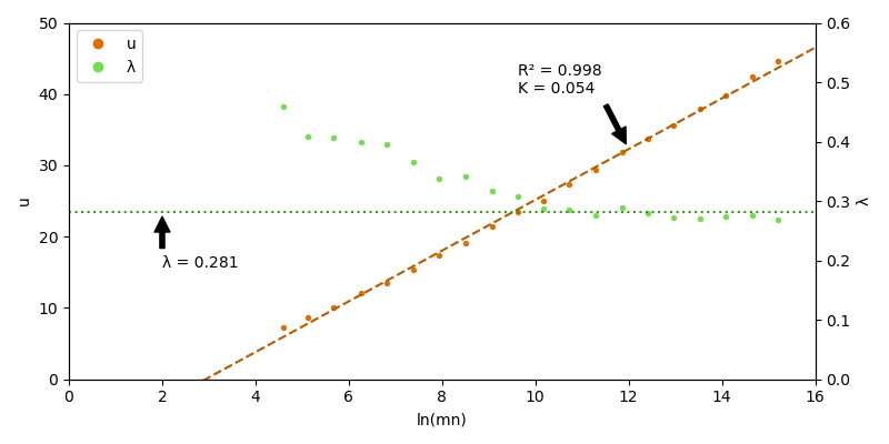
With a correlation of \(R^2 = 0.998\) we can assume that we can use the linear relation \(u = (\ln Kmn) / \lambda\). This allows use to sample \(K\) and \(\lambda\) at a single sequence length and use these parameters for all other local alignments with the same gap penalty, substitution matrix and background frequencies.

However, \(\lambda\) is not constant in this experiment: For rather short sequence lengths (\(< \sim 100\)) the obtained \(\lambda\) from the fit is significantly underestimated. There is the possibility to mitigate this error via edge correction 1, but keep in mind that the estimated \(\lambda\) is valid for the asymptotic case (very large sequences) and gets inaccurate for alignments of short sequences.

E-value calculation

Finally, we can use the estimated parameters to calculate the E-value of the alignment of interest. In this case we use \(K\) and \(\lambda\) from the linear fit, but as already indicated we could alternatively use the parameters from sampling alignments of sequences at a single length \(n\). While \(\lambda\) is a direct result of the method of moments as shown above, \(K\) is calculated as

\[K = \frac{e^{\lambda u}}{n^2}\]

where \(n\) is the length of both sequences in each sample.

The formula for the E-value is \(E = Kmn e^{-\lambda s}\) as shown above, where \(m\) and \(n\) are the sequence lengths. We can set \(m\) to the length of the query sequence, but for \(n\) there are two possibilities: Either you take the summed lengths of all sequences in the database or you take the length of the hit sequence multiplied with the number of sequences in the database. Here we go with the second option and assume that your hypothetical database contains a million sequences.

DATABASE_SIZE = 1_000_000

def e_value(score, length1, length2, k, l):
    return k * length1 * length2 * np.exp(-l * score)

e = e_value(
    alignment.score, len(query_seq), len(hit_seq) * DATABASE_SIZE, k, l
)
print(f"E-value = {e:.2e}")

E-value = 1.32e-07

With this low E-value, the homology between your avidin query sequence and the streptavidin hit sequence is highly significant. The result of this hypothetical database search is expected, since avidin and streptavidin have a high structural similarity and a similar function, namely binding the small molecule biotin.

References

1(1,2)

S. F. Altschul, W. Gish, “Local alignment statistics,” Methods in Enzymology, vol. 266, pp. 460–480, January 1996. doi: 10.1016/S0076-6879(96)66029-7

2

A. B. Robinson, L. R. Robinson, “Distribution of glutamine and asparagine residues and their near neighbors in peptides and proteins.,” Proceedings of the National Academy of Sciences, vol. 88, pp. 8880–8884, October 1991. doi: 10.1073/pnas.88.20.8880

3

S. F. Altschul, B. W. Erickson, “A nonlinear measure of subalignment similarity and its significance levels,” Bulletin of Mathematical Biology, vol. 48, pp. 617–632, September 1986. doi: 10.1007/BF02462327